an optimal algorithm for relay node assignment in cooperative ad hoc networks

1
An Optimal Algorithm for Relay Node Assignment
in Cooperative Ad Hoc Networks
Sushant Sharma, Student Member, IEEE, Yi Shi, Member, IEEE, Y. Thomas Hou, Senior Member, IEEE,
Sastry Kompella, Member, IEEE
Abstract—Recently, cooperative communications, in the form
of having each node equipped with a single antenna and exploit
spatial diversity via some relay node’s antenna, is shown to
be a promising approach to increase data rates in wireless
networks. Under this communication paradigm, the choice of
a relay node (among a set of available relay nodes) is critical
in the overall network performance. In this paper, we study the
relay node assignment problem in a cooperative ad hoc network
environment, where multiple source-destination pairs compete
for the same pool of relay nodes in the network. Our objective is
to assign the available relay nodes to different source-destination
pairs so as to maximize the minimum data rate among all pairs.
The main contribution of this paper is the development of an
optimal polynomial time algorithm, called ORA, that achieves
this objective. A novel idea in this algorithm is a “linear marking”
mechanism, which maintains linear complexity of each iteration.
We give a formal proof of optimality for ORA and use numerical
results to demonstrate its capability.
Index Terms—Cooperative communications, relay node assign-
ment, achievable rate, ad hoc network, optimization.
I. INTRODUCTION
S
PATIAL diversity, in the form of employing multiple
transceiver antennas, is shown to be very effective in
coping fading in wireless channel. However, equipping a wire-
less node with multiple antennas may not be practical, as the

footprint of multiple antennas may not fit on a wireless node
(particularly on a handheld wireless device). To achieve spatial
diversity without requiring multiple transceiver antennas on
the same node, the so-called cooperative communications has
been introduced [10], [16], [17]. Under cooperative communi-
cations, each node is equipped with only a single transceiver
and spatial diversity is achieved by exploiting the antenna on
another (cooperative) node in the network.
We consider two categories of cooperative communications,
namely, amplify-and-forward (AF) and decode-and-forward
(DF) [10]. Under AF, the cooperative relay node amplifies the
signal received from the information source before forwarding
Manuscript received May 26, 2009; revised January 29, 2010 and August
23, 2010; approved by IEEE/ACM TRANSACTIONS ON NETWORKING Editor
S. Diggavi.
An abridged version of this paper was published in ACM MobiHoc 2008
under the title “Optimal Relay Assignment for Cooperative Communications”.
S. Sharma is with the Department of Computer Science, Virginia Poly-
technic Institute and State University, Blacksburg, VA 24061 USA (e-mail:
).
Y. Shi and Y.T. Hou are with the Bradley Department of Electrical and
Computer Engineering, Virginia Polytechnic Institute and State University,
Blacksburg, VA 24061 USA e-mail: (; ).
S. Kompella is with the Information Technology Division, US
Naval Research Laboratory, Washington, DC 20375 USA (e-mail: kom-
).
it to the destination node. Under DF, the cooperative relay
node decodes the received signal, and re-encodes it before
forwarding it to the destination node. Regardless of AF or
DF, the choice of a relay node plays a critical role in the

performance of cooperative communications [1], [2], [24]. As
we shall see in Section III, an improperly chosen relay node
may offer a smaller data rate for a source-destination pair than
that under direct transmission.
In this paper, we study the relay node assignment problem
in a cooperative ad hoc network environment. Specifically,
we consider an ad hoc network where there are multiple
active source-destination pairs and the remaining nodes can be
exploited as relay nodes. We want to determine the optimal
assignment of relay nodes to the source-destination pairs so as
to maximize the minimum data rate among all pairs. Although
solution to this problem can be found via exhaustive search
(among all possible relay node assignments), the complexity
is exponential. Our goal in this paper is to find an algorithm
with polynomial-time complexity to solve this problem.
A. Main Contributions
In this paper, we study how to assign a set of relay nodes
to a set of source-destination pairs so as to maximize the
minimum achievable data rate among all the pairs. The main
contributions of this paper are the following.
• We develop an algorithm, called Optimal Relay Assign-
ment (ORA) algorithm, to solve the relay node assign-
ment problem. A novel idea in ORA is a “linear marking”
mechanism, which is able to offer a linear complexity at
each iteration. Due to this mechanism, ORA is able to
achieve polynomial time complexity.
• We offer a formal proof of optimality for the ORA
algorithm. The proof is based on contradiction and hinges
on a clever recursive trace-back of source nodes and relay
nodes in the solution by ORA and another hypothesized

better solution.
• We show a number of nice properties associated with
ORA. These include: (i) the algorithm works regardless
of whether the number of relay nodes in the network is
more than or less than the number of source-destination
pairs; (ii) the final achievable rate for each source-
destination pair is guaranteed to be no less than that
under direct transmissions; (iii) the algorithm is able to
find the optimal objective regardless of initial relay node
assignment.
2
• We provide a sketch of a possible implementation of the
ORA algorithm. Some practical issues and overhead in
the implementation are discussed.
B. Paper Organization
In Section II, we discuss related work and contrast them
with this paper. Section III gives a brief overview of coopera-
tive communications, so as to set the context of our study. In
Section IV, we describe the relay node assignment problem
in a cooperative ad hoc network environment. Section V
presents our ORA algorithm. In Section VI, we give a proof
of optimality for ORA. Section VII presents numerical results,
and Section VIII presents a sketch of how ORA can be
implemented. Section IX concludes this paper.
II. RELATED WORK
The concept of cooperative communications can be traced
back to the three-terminal communication channel (or a relay
channel) in [20] by Van Der Meulen. Shortly after, Cover and
El Gamal studied the general relay channel and established an
achievable lower bound for data transmission [4]. These two

seminal works laid down the foundation for the present-day
research on cooperative communications that can be broadly
classified into the following three categories.
(a) Physical Layer Schemes. Current research on CC aims
to exploit distributed antennas on other nodes in the network.
This has resulted in several protocols at the physical layer [5],
[7], [8], [10], [14], [16], [17]. These protocols describe various
ways through which nodes can cooperate at the physical layer.
In [10], Laneman et al. studied the mutual information
between a pair of nodes using a third cooperating node
under the so-called fixed relaying schemes (AF or DF). The
underlying physical layer model for CC in this paper is based
on these two schemes. In addition to fixed relaying schemes,
the authors also presented selection relaying, in which nodes
can switch between AF or DF (depending on instantaneous
channel conditions), and incremental relaying, which utilizes
limited feedback from the receiving node to further improve
the performance of CC.
In [7], Gunduz and Erkip studied an opportunistic coopera-
tion scheme in which a feedback channel among cooperating
nodes can be used to share channel state information and
help perform power control. The authors showed that the
performance of DF improves when power control is employed.
This kind of opportunistic DF is an alternative to the physical
layer fixed DF considered in our work.
Another alternative physical layer scheme could be the
delay-tolerant DF presented in [5]. In this delay-tolerant DF
scheme, distributed space-time codes are used to address the
issue of asynchrony (transmission delay) among cooperative
transmitters.

Additionally, in [8] and [14], authors studied multi-hop
cooperative protocols that involve cooperation among multiple
transmitting nodes along the path. In [16] and [17], the
authors performed an in-depth study on the practical issues
of implementing user cooperation in a conventional CDMA
system.
(b) Network Layer Schemes for Multi-hop Networks.
Recent efforts on CC at the network layer include [9], [15],
[22]. In [9], Khandani et al. studied minimum energy routing
problem (for a single message) by exploiting both wireless
broadcast advantage and CC. However, their proposed solu-
tions cannot provide any performance guarantee for general
ad hoc networks. In [22], Yeh and Berry aimed to generalize
the well known maximum differential backlog policy [18] in
the context of CC. They formulated a challenging nonlinear
program with exponential number of variables that character-
izes the network stability region, but only provided solutions
for a few simple network topologies. In [15], Scaglione et al.
proposed two architectures for multi-hop cooperative wireless
networks. Under these architectures, nodes in the network
can form multiple cooperative clusters. They showed that
the network connectivity can be improved by using such
cooperative clusters. However, problems related with optimal
routing and relay node assignment were not discussed in their
work.
(c) Relay Node Assignment for Ad hoc Networks. The
most relevant research to our work (i.e. relay node assignment)
include [1], [2], [13], [21], [24]. In [24], Zhao et al. showed
that for a single source-destination pair, in the presence of
multiple relay nodes, it is sufficient to choose one “best”

relay node, instead of multiple relay nodes. This result is
interesting, as it paves the way for research on assigning no
more than one relay node to a source-destination pair, which
is the setting that we have adopted in this paper. In [21],
Wang et al. showed how game theory can be used by a
single session to select the best cooperative relay node. In [1],
Bletsas et al. proposed a distributed scheme for relay node
selection based on the instantaneous channel conditions at the
relay node. In contrast to [1], [21], and [24], our paper is
not limited to a single-session, and considers the relay node
assignment for multiple competing sessions with the goal of
maximizing the minimum data rate among all of them. In [13],
Ng and Yu studied an important utility maximization problem
for the joint optimization of relay node selection, cooperative
communications, and resource allocation in a cellular network.
However, their solution procedure has non-polynomial running
time. In [2], Cai et al. studied relay node selection and power
allocation for AF-based wireless relay networks, and proposed
a heuristic solution. Additionally, both [2] and [13] have
different objectives from our work.
III. COOPERATIVE COMMUNICATIONS: A PRIMER
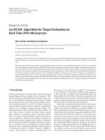
The essence of cooperative communications is best ex-
plained by a three-node example in Fig. 1. In this figure, node
s is the source node, node d is the destination node, and node
r is a relay node. Transmission from s to d is done on a frame-
by-frame basis. Within a frame, there are two time slots. In
the first time slot, source node s makes a transmission to the
destination node d. Due to the broadcast nature of wireless
communications, this transmission is also overheard by the
relay node r. In the second time slot, node r forwards the

data received in the first time slot to node d. Note that such a
two-slot structure is necessary for cooperative communications
due to the half-duplex nature of most wireless transceivers.
3
r
s
d
Fig. 1. A three-node schematic for cooperative communication.
In this section, we give expressions for achievable data rate
under cooperative communications and direct transmissions
(i.e., no cooperation). For cooperative communications, we
consider both amplify-and-forward (AF) and decoded-and-
forward (DF) modes [10].
Amplify-and-Forward (AF) Under this mode, let h
sd
, h
sr
,
h
rd
capture the effects of path-loss, shadowing, and fading
between nodes s and d, s and r, and r and d, respectively.
Denote z
d
[1] and z
d
[2] the zero-mean background noise at
node d in the first time slot and second time slot, respectively,
both with variance σ
2

d
. Denote z
r
[1] the zero-mean background
noise at node r in the first time slot, with variance σ
2
r
.
Denote x
s
the signal transmitted by source node s in the
first time slot. Then the received signal at destination node d,
y
sd
, can be expressed as
y
sd
= h
sd
x
s
+ z
d
[1] , (1)
and the received signal at the relay node r, y
sr
, is
y
sr
= h

sr
x
s
+ z
r
[1] . (2)
In the second time slot, relay node r transmits to destination
node d. The received signal at d, y
rd
, can be expressed as
y
rd
= h
rd
· α
r
· y
sr
+ z
d
[2] ,
where α
r
is the amplifying factor at relay node r and y
sr
is
given in (2). Thus, we have
y
rd
= h

rd
α
r
· (h
sr
x
s
+ z
r
[1]) + z
d
[2] . (3)
The amplifying factor α
r
at relay node r should satisfy power
constraint α
2
r
(|h
sr
|
2
P
s
+ σ
2
r
) = P
r
, where P

s
and P
r
are the
transmission powers at nodes s and r, respectively. So, α
r
is
given by
α
2
r
=
P
r
|h
sr
|
2
P
s
+ σ
2
r
.
We can re-write (1), (2) and (3) into the following compact
matrix form
Y = Hx
s
+ BZ ,
where

Y =

y
sd
y
rd

, H =

h
sd
α
r
h
rd
h
sr

,
B =

0 1 0
α
r
h
rd
0 1

, and Z =



z
r
[1]
z
d
[1]
z
d
[2]


. (4)
It has been shown in [10] that the above channel, which
combines both direct path (s to d) and relay path (s to r to d),
can be modeled as a one-input, two-output complex Gaussian
noise channel. The achievable data rate C
AF
(s, r, d) from s to
d can be given by
C
AF
(s, r, d) =
W
2
log
2
[det(I + (P
s
HH

†
)(BE[ZZ
†
]B
†
)
−1
)] ,
(5)
where W is the bandwidth, det(·) is the determinant function,
I is the identity matrix, the superscript “†” represents the
complex conjugate transposition, and E[·] is the expectation
function.
After putting (4) into (5) and performing algebraic ma-
nipulations, we have C
AF
(s, r, d) =
W
2
log

1 +
P
s
σ
2
d
|h
sd
|

2
+
P
s
|h
sr
|
2
P
r
|h
rd
|
2
P
s
σ
2
d
|h
sr
|
2
+ P
r
σ
2
r
|h
rd

|
2
+ σ
2
r
σ
2
d

. Denote SNR
sd
=
P
s
σ
2
d
|h
sd
|
2
, SNR
sr
=
P
s
σ
2
r
|h

sr
|
2
, and SNR
rd
=
P
r
σ
2
d
|h
rd
|
2
. We
have
C
AF
(s, r, d) = W · I
AF
(SNR
sd
, SNR
sr
, SNR
rd
) , (6)
where I
AF

(SNR
sd
, SNR
sr
, SNR
rd
) =
1
2
log
2

1 + SNR
sd
+
SNR
sr
·SNR
rd
SNR
sr
+SNR
rd
+1

.
Decode-and-Forward (DF) Under this mode, relay node r
decodes and estimates the received signal from source node s
in the first time slot, and then transmits the estimated data to
destination node d in the second time slot. The achievable data

rate for DF under the two time-slot structure is given by [10]
as
C
DF
(s, r, d) = W · I
DF
(SNR
sd
, SNR
sr
, SNR
rd
) , (7)
where
I
DF
(SNR
sd
, SNR
sr
, SNR
rd
) =
1
2
min{log
2
(1 + SNR
sr
),

log
2
(1 + SNR
sd
+ SNR
rd
)}. (8)
Note that I
AF
(·) and I
DF
(·) are increasing functions of P
s
and P
r
, respectively. This suggests that, in order to achieve the
maximum data rate under either mode, both source node and
relay node should transmit at maximum power. In this paper,
we let P
s
= P
r
= P .
Direct Transmission When cooperative communications
(i.e., relay node) is not used, source node s transmits to
destination node d in both time slots. The achievable data rate
from node s to node d is
C
D
(s, d) = W log

2
(1 + SNR
sd
) .
Based on the above results, we have two observations.
First, comparing C
AF
(or C
DF
) to C
D
, it is hard to say that
cooperative communications is always better than the direct
transmission. In fact, a poor choice of relay node could make
the achievable data rate under cooperative communications to
be lower than that under direct transmission. This fact under-
lines the significance of relay node selection in cooperative
communications. Second, although AF and DF are different
mechanisms, the capacities for both of them have the same
form, i.e., a function of SNR
sd
, SNR
sr
, and SNR
rd
. Therefore,
a relay node assignment algorithm designed for AF is also
applicable for DF. In this paper, we develop a relay node
assignment algorithm for both AF and DF. Table I lists the
notation used in this paper.

4
TABLE I
NOTATION
Symbol Definition
C
R
(s
i
, r
j
) Achievable rate for s
i
-d
i
pair when relay node r
j
is
used
C
R
(s
i
, ∅) Achievable rate for s
i
-d
i
pair under direct transmission
C
min
The minimum rate among all source-destination

pairs
h
uv
Effect of path-loss, shadowing, and fading from node
u to node v
N
s
Set of source nodes in the network
N
r
Set of relay nodes in the network
N
s
= |N
s
|, number of source nodes in the network
N
r
= |N
r
|, number of relay nodes in the network
N Number of all the nodes in the network
P Maximum transmission power
r
j
The j-th relay node, r
j
∈ N
r
R

ψ
(s
i
) The relay node assigned to s
i
under ψ
s
i
The i-th source node, s
i
∈ N
s
S
ψ
(r
j
) The source node that uses r
j
under ψ
SNR
uv
The signal noise ratio between nodes u and v
W Channel bandwidth
x
s
Signal transmitted by node s
y
uv
Received signal at node v (form node u)
z

v
[t] Background noise at node v during time slot t
α
r
Amplifying factor at relay r
σ
2
v
Variance of background noise at node v
ψ A solution for relay node assignment
IV. THE RELAY NODE ASSIGNMENT PROBLEM
Based on the background in the last section, we consider
relay node assignment problem in a network setting. There
are N nodes in an ad hoc network, with each node being
either a source node, a destination node, or a potential relay
node (see Fig. 2). In order to avoid interference, we assume
that orthogonal channels are available in the network (e.g.,
using OFDMA), which is proposed for cooperative communi-
cations [10]. The channel gain from node u to v is captured by
variable h
uv
. Denote N
s
= {s
1
, s
2
, · · ·, s
N
s

} the set of source
nodes, N
d
= {d
1
, d
2
, · · ·, d
N
d
} the set of destination nodes,
and N
r
= {r
1
, r
2
, · · · , r
N
r
} the set of relays (see Fig. 2). We
consider unicast transmission where every source node s
i
is
paired with a destination node d
i
, i.e., N
d
= N
s

. We also
consider that each node is equipped with a single transceiver
and can transmit/receive within one channel at a time. We
assume that each node can only serve a unique role of source,
destination, or relay. That is, N
r
= N − 2N
s
. Further, we
assume that a session utilizes one relay node for CC [24].
Note that a source node may not always get a relay node.
There are two possible scenarios in which this may happen.
First, there may not be sufficient number of relay nodes in the
network (e.g., N
r
< N
s
). In this case, some source nodes will
not have relay nodes. Second, even if there are enough relay
nodes, a sender may choose not to use a relay node if it leads
to a lower data rate than direct transmission (see discussion at
the end of Section III).
We now discuss the objective function of our problem.
Although different objectives can be used, a widely-used
objective for CC is to increase the achievable data rate of
individual sessions. For the multi-session network environment
considered in this paper (see Fig. 2), each source-destination
pair will have a different achievable data rate after we apply
a relay node assignment algorithm. So, a plausible objective
is to maximize the minimum data rate among all the source-

Sender
Receiver Potential Relay Node
Fig. 2. A cooperative ad hoc network consisting of source nodes, destination
nodes, and relay nodes.
destination pairs.
More formally, denote R(s
i
) the relay node assigned to s
i
,
and S(r
j
) as the source node that uses r
j
. For both AF and
DF, the achievable data rate of the session can be written as
(see Section III)
W I
R
(SNR
s
i
,d
i
, SNR
s
i
,R(s
i
)

, SNR
R(s
i
),d
i
) ,
with I
R
(·) = I
AF
(·) when AF is employed, and I
R
(·) = I
DF
(·)
when DF is employed. In case s
i
does not use a relay, we
denote R(s
i
) = ∅, and the data rate is the achievable rate
under direct transmission, i.e.,
C
R
(s
i
, ∅) = C
D
(s
i

, d
i
) .
Combining both these cases, we have
C
R
(s
i
, R(s
i
)) =



W I
R
(SNR
s
i
,d
i
, SNR
s
i
,R(s
i
)
,
SNR
R(s

i
),d
i
) if R(s
i
) = ∅
W log(1 + SNR
s
i
,d
i
) if R(s
i
) = ∅
(9)
Note that we do not list d
i
in function C
R
(s
i
, R(s
i
)) since for
each source node s
i
, the corresponding destination node d
i
is
deterministic.

Denote C
min
as our objective function, which is the mini-
mum rate among all source nodes. That is,
C
min
= min{C
R
(s
i
, R(s
i
)) : s
i
∈ N
s
}.
Our objective is to find an optimal relay node assignment for
all the source-destination pairs such that C
min
is maximized.
In subsequent sections, we present a polynomial time so-
lution to the relay node assignment problem along with a
correctness proof.
V. AN OPTIMAL RELAY ASSIGNMENT ALGORITHM
A. Basic Idea
The optimal polynomial-time algorithm we will present is
called Optimal Relay Assignment (ORA) algorithm. Figure 3
shows the flow chart of the ORA algorithm.
Initially, the ORA algorithm starts with a random but

feasible relay node assignment. By feasible, we mean that
each source-destination pair can be assigned at most one relay
node and that a relay node can be assigned only once. Such
initial feasible assignment is easy to construct, e.g., direct
transmission between each source-destination pair (without the
use of a relay) is a special case of feasible assignment.
Starting with this initial assignment, ORA adjusts the as-
signment during each iteration, with the goal of increasing
the objective function C
min
. Specifically, during each iteration,
ORA identifies the source node that corresponds to C
min
.
5
BEGIN
Better solution found.
NO
YES
NO
Preprocessing, and
Initial relay assignment
Can we find
a better solution?
YES
NO
Start the search
Return
YES
Return

NO
END
YES
Mark this relay, and denote
its corresponding source as s
BEGIN
Find_Another_Relay(s )
YES
NO
Is this relay
already assigned?
Can we find an
unmarked relay for s
with data rate larger
than Cmin?
For s , use
Find_Another_Relay(s ) to
determine if another
relay can be
assigned
Identify the source s
with minimum data rate Cmin.
b
i
Clear marks on
all relays.
Use Find_Another_Relay(s ) to
improve the data rate of s ,
and return the outcome.
b

b
i
j
j
j
Fig. 3. A flow chart of the ORA algorithm.
Then, ORA helps this source node to search a better relay
such that this “bottleneck” data rate can be increased. In the
case that the selected relay is already assigned to another
source node, further adjustment of relay node for that source
node is necessary (so that its current relay can be released).
Such adjustment may have a chain effect on a number of
source nodes in the network. It is important that for any
adjustment made on a relay node, the affected source node
should still maintain a data rate larger than C
min
. There are
only two outcomes from such search in an iteration: (i) a better
assignment is found, in which case, ORA moves on to the next
iteration; or (ii) a better assignment cannot be found, in which
case, ORA terminates.
There are two key technical challenges we aim to address
in the design. First, for any non-optimal solution, the algo-
rithm should be able to find a better solution. As a result,
upon termination, the final assignment is optimal. Second,
its running time must be polynomial. We will show that
s
cannot find
another relay
3

s
4
r
4
s
2
r
2
6
r
1
r
3
5
5
6
7
cannot find
another relay
can be
assigned to
1
r
r
r
s
s
s
6
s

Fig. 4. An example tree topology in ORA algorithm for finding a better
solution.
ORA addresses both problems successfully. Specifically, we
show the complexity of the ORA algorithm is polynomial
in Section V-D. We will also give a correctness proof of its
optimality in Section VI.
B. Algorithm Details
In the beginning, ORA algorithm performs a “preprocess-
ing” step. In this step, for each source-destination pair, the
source node s
i
considers each relay node r
j
in the network
and computes the corresponding data rate C
R
(s
i
, r
j
) by (9).
Each source node s
i
also computes the rate C
R
(s
i
, ∅) by (9)
under direct transmissions (i.e., without the use of a relay
node). After these computations, each source node s

i
can
identify those relay nodes that can offer an increase in its
data rate compared to direct transmissions, i.e., those relays
with C
R
(s
i
, r
j
) > C
R
(s
i
, ∅). Obviously, it only makes sense to
consider these relays for CC. In the case that no relay can offer
any increase of data rate compared to direct transmissions, we
will just employ direct transmissions for these source nodes.
After the preprocessing step, we enter the initial assignment
step. The objective of this step is to obtain an initial feasible
solution for ORA algorithm so that it can start its iteration.
In the pre-processing step, we have already identified the list
of relay nodes for each source node that can increase its data
rate compared to direct transmission. We can randomly assign
a relay node from this list to a source node. Note that once a
relay node is assigned to a source node, it cannot be assigned
again to another source node. Thus, if there is no relay node
available to a source node, then this source node will simply
employ direct transmission as its initial assignment. Upon the
completion of this assignment, each source node will have the

data rate no less than that under direct transmission.
The next step in the ORA algorithm is to find a better
assignment, which represents an iteration process. This is the
key step in the ORA algorithm. The detail of this step is shown
in the bottom portion of Fig. 3. As a starting point of this step,
ORA algorithm identifies the smallest data rate C
min
among
all sources. ORA algorithm aims to increase this minimum
rate for the corresponding source node, while having all other
source nodes maintain their data rates above C
min
. Without
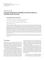
loss of generality, we use Fig. 4 to illustrate a search process.
• Suppose ORA identifies that s
1
has the smallest rate C
min
under the current assignment (with relay node r
1
). Then
6
s
1
examines other relays with a rate larger than C
min
. If it
cannot find such a relay, then no better solution is found
and the ORA algorithm terminates.
In case of a tie, i.e., when two or more source nodes have

the same smallest data rate, the tie is broken by choosing
the source node with the highest node index.
• Otherwise, i.e., if there are better relays, we consider
these relays in the non-increasing order in terms of data
rate (should it be assigned to s
1
). That is, we try the relay
that can offer the maximum possible increase in data rate
first. In case of a tie, i.e., when two or more relay nodes
offer the same maximum data rate, the tie is broken by
choosing the relay node with the highest node index.
• Suppose that source node s
1
considers relay node r
2
. If
this relay node is not yet assigned to any other source
node, then r
2
can be immediately assigned to s
1
. In this
simple case, we find a better solution and the current
iteration is completed.
• Otherwise, i.e., r
2
is already assigned to a source node,
say s
2
, we mark r

2
to indicate that r
2
is “under consid-
eration” and check whether r
2
can be released by s
2
.
• To release r
2
, source node s
2
needs to find another relay
(or use direct transmission) while making sure that such
new assignment still has its data rate larger than C
min
.
This process is identical to what we have done for s
1
,
with the only (but important) difference that s
2
will not
consider a relay that has already been “marked”, as that
relay node has already been considered by a source node
encountered earlier in the search process of this iteration.
• Suppose that source node s
2
now considers relay r

3
. If
this relay node is not yet assigned to any source node,
then r
3
can be assigned to s
2
; r
2
can be assigned to s
1
;
and the current iteration is completed. Moreover, if the
relay under consideration by s
2
is the one that is being
used by the source node that initiated the iteration, i.e.,
relay r
1
, then it is easy to see that r
1
can be taken away
from s
1
. A better solution, where r
1
is assigned to s
2
,
and r

2
is assigned to s
1
, is found and the current iteration
is completed. Otherwise, we mark r
3
and check further
to see whether r
3
can be released by its corresponding
source node, say s
3
. We also note that s
2
can consider
direct transmission if it offers a data rate larger than C
min
.
• Suppose that s
3
cannot find any “unmarked” relay that
offers a data rate larger than C
min
, and its data rate under
direct transmission is no more than C
min
. Then s
2
cannot
use r

3
as its relay.
• If any “unmarked” relay that offers a data rate larger
than C
min
cannot be assigned to s
2
, then s
1
cannot use
r
2
and will move on to consider the next relay on its
non-increasing rate list, say r
4
.
• The search continues, with relay nodes being marked
along the way, until a better solution is found or no better
solution can be found. For example, in Fig. 4, s
6
finds
a new relay r
7
. As a result, we have a new assignment,
where r
7
is assigned to s
6
; r
6

is assigned to s
4
; and r
4
is assigned to s
1
.
Note that the “mark” on a relay node will not be cleared
Main algorithm
1. Perform preprocessing and an initial relay node assignment.
2. Set all the relay nodes in the network as “unmarked”.
3. Denote s
b
the source node with C
min
,

the smallest data
rate among all source nodes. The corresponding destination
node of s
b
is d
b
and the corresponding relay node is R(s
b
).
4. Find Another Relay (s
b
, R(s
b

), C
min
).
5. If s
b
finds a better relay, then go to line 2.
6. Otherwise, the algorithm terminates.
Subroutines
Find Another Relay(S(r
j
), r
j
, C
min
):
7. For every “unmarked” relay r
k
with C
R
(S(r
j
), r
k
) > C
min
,
do the following in the non-increasing order of C
R
(S(r
j

), r
k
).

8. Run Check Relay Availability(r
k
, C
min
).
9. If r
k
is available, then do the following:
10. Remove relay node r
j
’s assignment to S(r
j
);
11. Assign relay node r
k
to S(r
j
).
12. Otherwise, continue on to next r
k
and go to line 8.
13. If all relays are unavailable, then S(r
j
) cannot find another relay.
Check Relay Availability(r
j

, C
min
):
14. If r
j
is not assigned to any source node, then r
j
is available.
15. If r
j
= R(s
b
) or r
j
= ∅, then r
j
is available.
16. Otherwise,
17. Set r
j
as “marked”.
18. Run Find Another Relay (S(r
j
), r
j
, C
min
).
19. If S(r
j

) can find another relay, then r
j
is available.
20. Otherwise r
j
is unavailable.

A tie is broken by choosing the node with the largest node index.
Fig. 5. Pseudocode for the ORA algorithm.
throughout the search process in the same iteration. We call
this the “linear marking” mechanism. These marks will only
be cleared when the current iteration terminates and before
the start of the next iteration. A pseudocode for the ORA
algorithm is shown in Fig. 5.
We now use an example to illustrate the operation of the
ORA algorithm, in particular, its “linear marking” mechanism.
Readers who already understood the ORA algorithm can skip
this example.
Example 1: Suppose that there are seven source-destination
pairs and seven relay nodes in the network.
Table II(a) shows the data rate for each source node s
i
when relay node r
j
is assigned to it. The symbol ∅ indicates
direct transmission. Also shown in Table II(a) is an initial
relay node assignment, which is indicated by an underscore
on the intersecting row (s
i
) and column (r

j
). Note that the
preprocessing step before the initial assignment ensures that
the data rate for each source-destination pair in the initial
assignment is no less than that under direct transmission.
Under the initial relay node assignment in Table II(a), source
s
3
is identified as the bottleneck source node s
b
with the
smallest rate of C
min
= 13. Since consideration of relay nodes
is performed in the order of non-increasing (from largest to
smallest) data rate for the source node under consideration,
r
4
is therefore considered for s
3
. Since r
4
is already assigned
to source node s
2
, we “mark” r
4
now. Now s
2
needs to find

another relay. But any other relay (or direct transmission) will
result in a data rate no greater than the current objective value
C
min
= 13. This means that r
4
cannot be taken away from s
2
.
Since r
4
does not work out for s
3
, s
3
will then consider the
next relay node that offers the second largest data rate value,
i.e., relay node r
7
. Since r
7
is already assigned to sender s
4
,
we “mark” r
7
now. Next, ORA algorithm will check to see if
s
4
can find another relay. It turns out that none of the relay

7
TABLE II
AN EXAMPLE.
(a) Initial relay node assignment.
∅ r
1
r
2
r
3
r
4
r
5
r
6
r
7
s
1
14 7 24 5 14 15 17 9
s
2
9 8 10 11 20 10 12 11
→ s
3
11 10 13 17 21 8 9 19
s
4
12 8 9 12 11 10 9 18

s
5
10 9 18 19 24 9 13 23
s
6
7 18 12 6 11 11 17 20
s
7
16 1 9 4 14 19 8 12
(b) Assignment after the first iteration.
∅ r
1
r
2
r
3
r
4
r
5
r
6
r
7
→ s
1
14 7 24 5 14 15 17 9
s
2
9 8 10 11 20 10 12 11

s
3
11 10 13 17 21 8 9 19
s
4
12 8 9 12 11 10 9 18
s
5
10 9 18 19 24 9 13 23
s
6
7 18 12 6 11 11 17 20
s
7
16 1 9 4 14 19 8 12
(c) Assignment after the second iteration.
∅ r
1
r
2
r
3
r
4
r
5
r
6
r
7

s
1
14 7 24 5 14 15 17 9
s
2
9 8 10 11 20 10 12 11
s
3
11 10 13 17 21 8 9 19
s
4
12 8 9 12 11 10 9 18
s
5
10 9 18 19 24 9 13 23
s
6
7 18 12 6 11 11 17 20
→ s
7
16 1 9 4 14 19 8 12
(d) Final assignment upon termination.
∅ r
1
r
2
r
3
r
4

r
5
r
6
r
7
s
1
14 7 24 5 14 15 17 9
s
2
9 8 10 11 20 10 12 11
→ s
3
11 10 13 17 21 8 9 19
s
4
12 8 9 12 11 10 9 18
s
5
10 9 18 19 24 9 13 23
s
6
7 18 12 6 11 11 17 20
s
7
16 1 9 4 14 19 8 12
nodes except r
7
can offer a data rate larger than the current

C
min
to s
4
. As a result, r
7
cannot be taken away from s
4
.
Source node s
3
will now check for the relay node that offers
next largest rate, i.e., r
3
. Since r
3
is already assigned to sender
s
5
, we “mark” r
3
now. Next, ORA algorithm checks to see if
s
5
can find another relay. Then s
5
checks relay nodes in non-
increasing order of data rate values. Since r
4
(with largest

rate), r
7
(with the second largest rate), and r
3
(with the third
largest rate) are all marked, they will not be considered. The
relay with the fourth largest rate is r
2
, which offers a rate of
18 > C
min
= 13. Moreover, r
2
is the relay node assigned to
s
b
= s
3
. Thus, s
5
can choose r
2
. The new assignment after
the first iteration is shown in Table II(b). Now the objective
value, C
min
, is updated to 15, which corresponds to s
1
. Before
the second iteration, all markings done in the first iteration are

cleared.
In the second iteration, ORA algorithm will identify s
1
as
the source node with a minimum data rate in the network.
The algorithm will then perform a new search for a better
relay node for source s
1
. Similar to the first iteration, the
assignments for other source nodes can change during this
search process, but all assignments should result in data rates
larger than 15.
The iteration continues and the final assignment upon ter-
mination of ORA algorithm is shown in Table II(d), with the
optimal (maximum) value of C
min
being 17.
It should be clear that ORA works regardless of whether
N
r
≥ N
s
or N
r
< N
s
. For the latter case, i.e., the number of
relay nodes in the network is less than the number of source
nodes, it is only necessary to consider relay node assignment
for a reduced subset of N

r
source nodes, where the data rate
of each source in this subset under direct transmission is less
than the data rate of those (N
s
− N
r
) source nodes not in this
subset. As a result, in the case of N
s
> N
r
, ORA will run
even faster due to a smaller problem size.
C. Caveat on the Proposed Marking Mechanism
We now re-visit the marking mechanism in the ORA
algorithm. Although different marking mechanisms may be
designed to achieve the optimal objective, the algorithm
complexity under different marking mechanisms may differ
significantly. In this section, we first present a marking mech-
anism, which appears to be a natural approach but leads to an
exponential complexity for each iteration. Then we discuss our
proposed marking mechanism and show its linear complexity
for each iteration.
A natural approach is to perform both marking and un-
marking within an iteration. This approach is best explained
with an example. Again, let’s look at Fig. 4. Source node
s
1
first considers r

2
. Since r
2
is being considered by s
1
in
the new solution and is used by s
2
in the current solution,
r
2
is marked. Source node s
2
considers r
3
, which is already
assigned to s
3
. Since s
3
cannot release r
3
without reducing
its data rate below the current C
min
, this branch of search is
futile and s
1
now considers a different relay node r
4

. Since
r
4
is currently assigned to s
4
, we mark r
4
and try to find a
new relay for s
4
. Now the question is: shall we remove those
marks on r
2
and r
3
that we put on earlier in the process within
this iteration? Under this natural approach, r
2
and r
3
should
be unmarked so that they can be considered as candidate
relay nodes for s
4
in its search. Similarly, when we try to
find a relay for s
6
, relay nodes r
2
, r

3
, r
4
and r
5
should be
unmarked so that they can be considered as candidate relay
nodes for s
6
, in addition to r
7
. It is not hard to show that
such marking/unmarking mechanism will consider all possible
assignments and can guarantee to find an optimal solution
upon termination. However, the complexity of such approach
is exponential within each iteration.
In contrast, under the ORA algorithm, there is no unmarking
mechanism within an iteration. That is, relay nodes that are
marked earlier in the search process by some source nodes will
remain marked. As a result, any relay node will be considered
at most once in the search process, which leads to a linear
complexity for each iteration. Unmarking for all nodes is
performed only at the end of an iteration so that there is a
clean start for the next iteration.
An immediate question regarding our marking mechanism
is: how could such a “linear marking” lead to an optimal
solution, as it appears that many possible assignments that may
increase C
min
are not considered. This is precisely the question

that we will address in Section VI, where we will prove that
ORA can guarantee that its final solution is optimal.
8
D. Complexity Analysis
We now analyze the computational complexity of ORA
algorithm. During each iteration, due to the “linear marking”
mechanism in our algorithm, a relay node is checked for
its availability at most once. Thus, the complexity of each
iteration is O(N
r
).
Now we examine the maximum number of iterations that
ORA can execute. The number of improvements in data rate
that an individual source node can have is limited by N
r
.
As a result, in worst case, the number of iterations that
the algorithm can go through are O(N
s
N
r
). This makes the
overall complexity of ORA algorithm to be O(N
s
N
2
r
).
VI. PROOF OF OPTIMALITY
In this section, we give a correctness proof of the ORA

algorithm. That is, upon the termination of the ORA algorithm,
the solution (i.e., objective value and the corresponding relay
node assignment) is optimal.
Our proof is based on contradiction. Denote ψ the final
solution obtained by the ORA algorithm, with the objective
value being C
min
. For ψ, denote the relay node assigned to
source node s
i
as R
ψ
(s
i
). Conversely, for ψ, denote the source
node that uses relay node r
j
as S
ψ
(r
j
).
We now assume that there exists a solution
ˆ
ψ better than ψ.
That is, the objective value by
ˆ
ψ, denoted as
ˆ
C

min
, is greater
than that by ψ, i.e.,
ˆ
C
min
> C
min
. For
ˆ
ψ, we denote the relay
node assigned to source node s
i
as R
ˆ
ψ
(s
i
). Conversely, for
ˆ
ψ,
we denote the source node that uses relay node r
j
as S
ˆ
ψ
(r
j
).
The key idea in the proof is to exploit the marking status

of relay nodes at the end of its last iteration, which is a non-
improving iteration. Specifically, in the beginning of this last
iteration, ORA will select a “bottleneck” source node, which
we denote as s
b
. ORA will then try to improve the solution
by searching for a better relay node for this bottleneck source
node. Since the last iteration is a non-improving iteration,
ORA will not find a better solution, and thus will terminate.
We will show that R
ψ
(s
b
) is not marked at the end of the last
iteration of ORA. On the other hand, by assuming that there
exists a better solution
ˆ
ψ than ψ, we will show that R
ψ
(s
b
)
will be marked at the end of the last iteration of ORA. This
leads to a contradiction and thus
ˆ
ψ cannot exist. We begin our
proof with the following fact.
Fact 1: For the bottleneck source node s
b
under ψ, its relay

node R
ψ
(s
b
) is not marked at the end of the last iteration of
the ORA algorithm.
Proof: In the ORA algorithm, a relay node r
j
is marked
only if r
j
= R
ψ
(s
b
) (see Check
Relay Availability() in
Fig. 5). Thus, R
ψ
(s
b
) cannot be marked at the end of the
last iteration of the ORA algorithm.
Fact 1 will be the basis for contradiction in our proof for
Theorem 1, the main result of this section.
Now we present the following three claims, which recur-
sively examine relay node assignment under
ˆ
ψ. First, for the
relay node assigned to s

b
in
ˆ
ψ, i.e., R
ˆ
ψ
(s
b
), we have the
following claim.
Claim 1: Relay node R
ˆ
ψ
(s
b
) must be marked at the end of
the last iteration of the ORA algorithm. Further, it cannot be
(marked)
^
^
^
^
n
G (s )
n
s
(unmarked)
(marked)
(marked)
(marked)

b
b
b
b
b
b
b
k
G (s )
k
b
b
^
R ( G (s ) )
R (s )
G (s )
R (s )
^
^
^
R ( G (s ) )
R ( G (s ) )
Fig. 6. The sequence of nodes under analysis in the proof of optimality.
∅ and must be assigned to some source node under solution
ψ.
Proof: Since
ˆ
ψ is a better solution than ψ, we have
C
R

(s
b
, R
ˆ
ψ
(s
b
)) ≥
ˆ
C
min
> C
min
. Thus, by construction, ORA
will consider the relay node R
ˆ
ψ
(s
b
)’s availability for s
b
in
its last iteration. Since ORA algorithm cannot find a better
solution in its last iteration, relay R
ˆ
ψ
(s
b
) should be marked
and then the outcome for checking R

ˆ
ψ
(s
b
)’s availability must
be unavailable. By “linear marking”, the mark on R
ˆ
ψ
(s
b
)
will not be cleared throughout the search process in the last
iteration. Thus, the relay node R
ˆ
ψ
(s
b
) is marked at the end
of the last iteration of ORA algorithm.
We now prove the second statement by contradiction. If
R
ˆ
ψ
(s
b
) is ∅, then s
b
will choose ∅ in the last iteration since
it can offer C
R

(s
b
, R
ˆ
ψ
(s
b
)) > C
min
. But this contradicts to
the fact that we are now in the last iteration of ORA, which
is a non-improving iteration. So R
ˆ
ψ
(s
b
) cannot be ∅. Further,
since we proved that R
ˆ
ψ
(s
b
) is marked at the end of the last
iteration of the ORA algorithm, it must be assigned to some
source node already.
By the definition of S
ψ
(·), we have that R
ˆ
ψ

(s
b
) is assigned
to source node S
ψ
(R
ˆ
ψ
(s
b
)) in solution ψ. To simplify nota-
tion, define function G
ψ
(·) as
G
ψ
(·) = S
ψ
(R
ˆ
ψ
(·)) . (10)
Thus, relay node R
ˆ
ψ
(s
b
) is assigned to source node G
ψ
(s

b
)
in ψ (see top portion of Fig. 6).
Since R
ˆ
ψ
(s
b
) = R
ψ
(s
b
), they are assigned to different
source nodes in ψ, i.e., G
ψ
(s
b
) = s
b
. Now, we recursively
investigate the relay node assigned to source G
ψ
(s
b
) under
solution
ˆ
ψ, i.e., R
ˆ
ψ

(G
ψ
(s
b
)). We have the following claim
(also see Fig. 6).
Claim 2: Relay node R
ˆ
ψ
(G
ψ
(s
b
)) must be marked at the
end of the last iteration of the ORA algorithm. Further, it
cannot be ∅ and must be assigned to some source node under
solution ψ.
The proofs for both statements in this claim follow the same
token as that for Claim 1.
9
Again, by the definition of S
ψ
(·), we have that relay node
R
ˆ
ψ
(G
ψ
(s
b

)) is assigned to source node S
ψ
(R
ˆ
ψ
(G
ψ
(s
b
))) in
solution ψ. By (10), we have source S
ψ
(R
ˆ
ψ
(G
ψ
(s
b
))) =
G
ψ
(G
ψ
(s
b
)). To simplify the notation, we define function
G
2
ψ

(·) as
G
2
ψ
(·) = G
ψ
(G
ψ
(·)) .
Thus, relay node R
ˆ
ψ
(G
ψ
(s
b
)) is assigned to source node
G
2
ψ
(s
b
) in ψ. Now we have two cases: source node G
2
ψ
(s
b
) may
or may not be a node in {s
b

, G
ψ
(s
b
)}. If source node G
2
ψ
(s
b
)
is a node in {s
b
, G
ψ
(s
b
)}, then we terminate our recursive
procedure. Otherwise, we can further consider its relay node
in
ˆ
ψ.
In general we can use the following notation.
G
0
ψ
(s
b
) = s
b
,

G
k
ψ
(s
b
) = G
ψ
(G
k−1
ψ
(s
b
)) (k ≥ 1). (11)
Since the numbers of source nodes are finite, our recursive
procedure will terminate in finite steps. Suppose that we
terminate at k = n.
Following the same token for Claims 1 and 2, we can
obtain a similar claim for each of the relay nodes R
ˆ
ψ
(G
2
ψ
(s
b
)),
R
ˆ
ψ
(G

3
ψ
(s
b
)), · · · , R
ˆ
ψ
(G
k
ψ
(s
b
)), ·· · , R
ˆ
ψ
(G
n
ψ
(s
b
)) (see Fig. 6).
Thus, we can generalize the statements in Claims 1 and 2 for
relay node R
ˆ
ψ
(G
k
ψ
(s
b

)) and have the following claim.
Claim 3: Relay node R
ˆ
ψ
(G
k
ψ
(s
b
)) must be marked at the
end of the last iteration of the ORA algorithm. Further, it
cannot be ∅ and must be assigned to some source node under
solution ψ, k = 0, 1, 2, · · · , n.
Proof: Since
ˆ
ψ is a better solution than ψ, we can say that
C
R
(G
k
ψ
(s
b
), R
ˆ
ψ
(G
k
ψ
(s

b
))) ≥
ˆ
C
min
> C
min
. Note that G
k
ψ
(s
b
) is
some source node in the solution ψ obtained by ORA, whereas
R
ˆ
ψ
(G
k
ψ
(s
b
)) is the relay node assigned to this source node in
the hypothesized better solution
ˆ
ψ. Our goal is to show that
ORA should have marked this relay node in its last iteration.
Since C
R
(G

k
ψ
(s
b
), R
ˆ
ψ
(G
k
ψ
(s
b
))) > C
min
and R
ˆ
ψ
(G
k
ψ
(s
b
)) is
not assigned to G
k
ψ
(s
b
) in the last iteration of ORA, then by
construction of ORA, ORA must have checked R

ˆ
ψ
(G
k
ψ
(s
b
))’s
availability for G
k
ψ
(s
b
) during the last iteration, then marked it,
and then determined it to be unavailable for G
k
ψ
(s
b
). Moreover,
due to “linear marking”, this mark on R
ˆ
ψ
(G
k
ψ
(s
b
)) should be
there after the last iteration of ORA. Thus, we can conclude

that R
ˆ
ψ
(G
k
ψ
(s
b
)) is marked at the end of the last iteration of
the ORA algorithm.
We now prove the second statement by contradiction. If
R
ˆ
ψ
(G
k
ψ
(s
b
)) is ∅, then G
k
ψ
(s
b
) will choose ∅ in the last iteration
since it can offer C
R
(G
k
ψ

(s
b
), R
ˆ
ψ
(G
k
ψ
(s
b
)) > C
min
, and finally
s
b
will be able to get a better relay node. But this contradicts
with the fact that this last iteration is a non-improving iteration.
So, R
ˆ
ψ
(G
k
ψ
(s
b
)) cannot be ∅. Further, since we proved that
R
ˆ
ψ
(G

k
ψ
(s
b
)) is marked at the end of the last iteration of the
ORA algorithm, it must be assigned to some source node
already.
Referring to Fig. 6, we have Claim 3 for a set of relay nodes
R
ˆ
ψ
(s
b
), R
ˆ
ψ
(G
ψ
(s
b
)), · · ·, R
ˆ
ψ
(G
n
ψ
(s
b
)). Our recursive proce-
dure terminates at R

ˆ
ψ
(G
n
ψ
(s
b
)) because its assigned source
node in solution ψ is a node in {s
b
, G
ψ
(s
b
), · · · , G
n
ψ
(s
b
)}. We
are now ready to prove the following theorem, which is the
main result of this section.
Theorem 1: Upon the termination of the ORA algorithm,
the obtained solution ψ is optimal.
Proof: Under Claim 3, we proved that the relay node
R
ˆ
ψ
(G
n

ψ
(s
b
)) is assigned to some source node in solution ψ
obtained by ORA. Since our recursive procedure terminates
at R
ˆ
ψ
(G
n
ψ
(s
b
)), its assigned source node in solution ψ is
a node in {s
b
, G
ψ
(s
b
), · · · , G
n
ψ
(s
b
)}. But we also know that
under ψ, source nodes G
ψ
(s
b

), G
2
ψ
(s
b
), G
3
ψ
(s
b
), · · ·, G
n
ψ
(s
b
)
have relay nodes R
ˆ
ψ
(s
b
), R
ˆ
ψ
(G
ψ
(s
b
)), R
ˆ

ψ
(G
2
ψ
(s
b
)), · · ·,
R
ˆ
ψ
(G
n−1
ψ
(s
b
)), respectively. Thus, R
ˆ
ψ
(G
n
ψ
(s
b
)) is the only
relay node that can be assigned to s
b
in solution ψ. On the
other hand, relay node assigned to s
b
in solution ψ is denoted

by R
ψ
(s
b
). Thus, we have R
ˆ
ψ
(G
n
ψ
(s
b
)) = R
ψ
(s
b
).
Now, Claim 3 states that R
ˆ
ψ
(G
n
ψ
(s
b
)) must be marked after
the last iteration, whereas Fact 1 states that the relay node
assigned to the bottleneck source node, i.e., R
ψ
(s

b
), cannot
be marked. Since both R
ψ
(s
b
) and R
ˆ
ψ
(G
n
ψ
(s
b
)) are the same
relay node, we have a contradiction. Thus our assumption that
there exists a solution
ˆ
ψ better than ψ does not hold. The proof
is complete.
Note that the proof of Theorem 1 does not depend on the
initial assignment in ORA. So we have the following important
property.
Corollary 1.1: Under any feasible initial relay node assign-
ment, the ORA algorithm can find an optimal relay node
assignment.
VII. NUMERICAL RESULTS
In this section, we present some numerical results to demon-
strate the properties of the ORA algorithm.
A. Simulation Setting

We consider a 100-node cooperative ad hoc network. The
location of each node is given in Table III. For this network, we
consider both the cases of N
r
≥ N
s
and N
r
< N
s
. In the first
case, we have 30 source-destination pairs and 40 relay nodes.
While in the second case, we have 40 source-destination pairs
and only 20 relay nodes. The role of each node (either as a
source, destination, or relay) for each case is shown in Figs. 7
and 9, respectively, with details given in Table III.
For the simulations, we assume W = 10 MHz bandwidth
for each channel. The maximum transmission power at each
node is set to 1 W. Each relay node employs AF for cooper-
ative communications. We assume that h
sd
only includes the
path loss component between nodes s and d and is given by
|h
sd
|
2
= ||s − d||
−4
, where ||s − d|| is the distance (in meters)

between these two nodes and 4 is the path loss index. Note
that the working of the ORA algorithm does not depend on the
mode of CC and the channel gain model. As long as channel
gains and achievable rates are known, ORA will give optimal
assignment. For the AWGN channel, we assume the variance
of noise is 10
−10
W at all nodes.
10
TABLE III
LOCATIONS AND ROLES OF ALL THE NODES IN THE NETWORK.
Node Role Node Role Node Role
Location Case 1 Case 2 Location Case 1 Case 2 Location Case 1 Case 2
(75, 500) s
1
s
1
(220, 190) d
4
d
4
(380, 370) r
7
s
31
(170, 430) s
2
s
2
(660, 190) d

5
d
5
(300, 350) r
8
r
8
(170, 500) s
3
s
3
(430, 630) d
6
d
6
(410, 650) r
9
s
33
(250, 650) s
4
s
4
(180, 620) d
7
d
7
(470, 500) r
10
d

40
(400, 550) s
5
s
5
(750, 625) d
8
d
8
(660, 525) r
11
s
39
(340, 230) s
6
s
6
(310, 480) d
9
d
9
(600, 425) r
12
s
40
(390, 150) s
7
s
7
(1100, 180) d

10
d
10
(510, 200) r
13
s
38
(460, 280) s
8
s
8
(1110, 360) d
11
d
11
(575, 325) r
14
r
14
(700, 500) s
9
s
9
(875, 600) d
12
d
12
(750, 560) r
15
r

15
(750, 360) s
10
s
10
(700, 300) d
13
d
13
(800, 360) r
16
r
16
(800, 90) s
11
s
11
(650, 550) d
14
d
14
(860, 260) r
17
r
17
(900, 160) s
12
s
12
(740, 170) d

15
d
15
(980, 450) r
18
r
18
(1125, 300) s
13
s
13
(410, 810) d
16
d
16
(950, 310) r
19
r
19
(1000, 340) s
14
s
14
(550, 1100) d
17
d
17
(950, 200) r
20
d

37
(1025, 540) s
15
s
15
(150, 790) d
18
d
18
(100, 1000) r
21
s
32
(100, 1120) s
16
s
16
(210, 1110) d
19
d
19
(310, 980) r
22
r
12
(150, 920) s
17
s
17
(530, 720) d

20
d
20
(250, 800) r
23
d
32
(330, 1110) s
18
s
18
(800, 1140) d
21
d
21
(460, 1010) r
24
r
13
(450, 890) s
19
s
19
(1080, 1100) d
22
d
22
(610, 930) r
25
d

34
(650, 1050) s
20
s
20
(940, 790) d
23
d
23
(680, 760) r
26
s
34
(700, 640) s
21
s
21
(1360, 640) d
24
d
24
(700, 900) r
27
r
20
(820, 880) s
22
s
22
(1280, 1120) d

25
d
25
(910, 1120) r
28
d
35
(1150, 1060) s
23
s
23
(1260, 350) d
26
d
26
(970, 970) r
29
s
35
(1480, 1120) s
24
s
24
(1500, 50) d
27
d
27
(1360, 910) r
30
r

9
(1160, 720) s
25
s
25
(1450, 605) d
28
d
28
(1200, 920) r
31
r
11
(1050, 50) s
26
s
26
(1030, 910) d
29
d
29
(1250, 690) r
32
d
36
(1350, 450) s
27
s
27
(1150, 230) d

30
d
30
(1290, 180) r
33
r
10
(1380, 110) s
28
s
28
(80, 370) r
1
d
31
(150, 360) r
34
r
5
(1500, 800) s
29
s
29
(110, 280) r
2
r
2
(1380, 380) r
35
r

7
(1500, 300) s
30
s
30
(160, 300) r
3
r
3
(1220, 60) r
36
s
37
(200, 50) d
1
d
1
(280, 520) r
4
r
4
(1190, 510) r
37
s
36
(520, 240) d
2
d
2
(375, 580) r

5
d
39
(500, 40) r
38
d
38
(40, 100) d
3
d
3
(385, 450) r
6
r
6
(50, 805) r
39
d
33
(1510, 920) r
40
r
1
400
s1
s3
s2
s4
s5
s6

s7
s8
s9
s15
s14
s10
s11
s12
s13
d3
d1
d7
d9
d2
d13
d15
d10
d4
d6
d14
d8
d12
d11
d5
r3
r1
r4
r8
r7
r6

r5
r9
r10
r11
r12
r13
r14
r15
r16
r18
r17
r19
r20
r2
0
800
Senders
Receivers
Potential Relays
100
200
300
500
600
700 800
900
1000
1100
1200
100

200
300
400
500
600
700
(meters)
(meters)
0
1300 1400
1500
1600
900
1000
1100
1200
s16
s17
s18
s19
s20
s21
s22
s23
s24
s25
s26
s27
s28
s29

s30
d16
d17
d18
d19
d20
d21
d22
d23
d24
d25
d26
d27
d28
d29
d30
r21
r22
r23
r24
r25
r26
r27
r28
r29
r30
r31
r32
r33
r34

r35
r36
r37
r38
r39
r40
Fig. 7. Topology for a 100-node network for Case 1 (N
r
≥ N
s
), with
N
s
= 30 and N
r
= 40.
B. Results
Case 1: N
r
≥ N
s
. In this case (see Fig. 7), we have 30
source-destination pairs and 40 relay nodes.
Under ORA, after preprocessing, we start with an initial
relay node assignment in the first iteration. Such initial as-
signment is not unique. But regardless of the initial relay
node assignment, we expect the objective value to converge
to the optimum (by Corollary 1.1). To validate this result, in
Table IV, we show the results of running the ORA algorithm
under two different initial relay node assignments, denoted as







Fig. 8. Case 1 (N
r
≥ N
s
): The objective value C
min
at each iteration of
ORA algorithm under two different initial relay node assignments.
I and II (see Table IV).
In Table IV, the second column shows the data rate for
each source-destination pair under direct transmissions. Note
that the minimum rate among all pairs is 1.83 Mbps, which
is associated with s
7
. The third to fifth columns are results
under initial relay node assignment I and sixth to eighth
columns are results under initial relay node assignment II.
The symbol ∅ denotes direct transmissions. Note that initial
relay node assignments I and II are different. As a result, the
final assignment is different under I and II. However, the final
11
TABLE IV
OPTIMAL ASSIGNMENTS FOR CASE 1 (N
r

≥ N
s
) UNDER TWO DIFFERENT
INITIAL RELAY NODE ASSIGNMENTS.
Relay Assignment I Relay Assignment II
Ses- C
D
Final Final
sion (Mbps) Initial Final Rate Initial Final Rate
(Mbps) (Mbps)
s
1
2.62 ∅ r
3
6.54 r
3
r
3
6.54
s
2
4.60 r
8
r
7
9.46 r
8
r
7
9.46

s
3
3.81 ∅ r
2
8.73 r
1
r
1
7.21
s
4
2.75 ∅ r
4
4.66 r
4
r
4
4.66
s
5
3.15 ∅ r
14
6.47 r
7
r
14
6.47
s
6
4.17 ∅ r

6
9.25 r
10
r
6
9.25
s
7
1.83 r
6
r
8
4.76 r
6
r
8
4.76
s
8
2.99 ∅ r
12
7.22 r
16
r
12
7.22
s
9
4.92 r
12

r
10
9.81 r
12
r
10
9.81
s
10
4.80 r
18
∅ 4.80 ∅ ∅ 4.80
s
11
4.13 r
16
r
20
9.13 r
17
r
20
9.13
s
12
3.23 ∅ r
19
5.89 r
18
r

18
5.55
s
13
3.68 ∅ r
18
4.84 r
19
r
17
7.32
s
14
4.23 ∅ r
16
7.87 r
15
r
15
5.29
s
15
2.62 r
17
r
17
4.86 r
20
r
19

5.84
s
16
3.30 ∅ r
22
7.29 r
22
r
22
7.29
s
17
4.17 ∅ r
24
5.62 r
24
r
24
5.62
s
18
6.03 r
21
r
21
7.37 r
23
r
23
6.26

s
19
8.76 ∅ ∅ 8.76 ∅ ∅ 8.76
s
20
6.95 ∅ ∅ 6.95 ∅ ∅ 6.95
s
21
1.90 r
27
r
27
4.90 r
27
r
27
4.90
s
22
7.65 r
28
r
28
8.71 r
28
r
28
8.71
s
23

7.55 r
29
r
29
11.26 r
29
r
28
11.26
s
24
2.12 r
40
r
40
4.43 ∅ r
40
4.43
s
25
3.90 ∅ r
30
5.87 ∅ r
30
5.87
s
26
6.08 r
36
r

36
6.81 r
36
r
36
6.81
s
27
3.61 ∅ r
34
5.44 ∅ r
34
5.44
s
28
2.04 r
35
r
35
5.29 ∅ r
35
5.29
s
29
2.32 r
30
r
31
4.68 ∅ r
31

4.68
s
30
6.60 r
34
r
33
9.65 r
34
r
33
9.65
400
s1
s3
s2
s4
s5
s6
s7
s8
s9
s15
s14
s10
s11
s12
s13
d3
d1

d7
d9
d2
d13
d15
d10
d4
d6
d14
d8
d12
d11
d5
r3
d31
r4
r8
s31
r6
d39
s33
d40
s39
s40
s38
r14
r15
r16
r18
r17

r19
d37
r2
0
Senders
Receivers
Potential Relays
100
200
300
500
600
700 800
900
1000
1100
1200
(meters)
(meters)
0
1300 1400
1500
1600
1100
1200
s16
s17
s18
s19
s20

s21
s22
s23
s24
s25
s26
s27
s28
s29
s30
d16
d17
d18
d19
d20
d21
d22
d23
d24
d25
d26
d27
d28
d29
d30
s32
r12
d32
r13
d34

s34
r20
d35
s35
r9
r11
d36
r10
r5
r7
s37
s36
d38
d33
r1
800
100
200
300
400
500
600
700
900
1000
Fig. 9. Topology for a 100-node network for Case 2 (N
r
< N
s
), with

N
s
= 40 and N
r
= 20.
objective value (i.e., C
min
) under I and II is identical (4.43
Mbps).
Figure 8 shows the objective value C
min
at each iteration
under initial relay node assignments I and II. Under either
initial relay node assignments I or II, C
min
is a non-decreasing
function of iteration number. Note that a higher initial value
of C
min
does not mean that ORA will converge faster. The
increase of C
min
by cooperative communications over direct
transmissions is significant (from 1.83 Mbps to 4.43 Mbps).
Case 2: N
r
< N
s
. In this case (see Fig. 9), we have 40
TABLE V

OPTIMAL ASSIGNMENTS FOR CASE 2 (N
r
< N
s
) UNDER TWO DIFFERENT
INITIAL RELAY NODE ASSIGNMENTS.
Relay Assignment I Relay Assignment II
Ses- C
D
Final Final
sion (Mbps) Initial Final Rate Initial Final Rate
(Mbps) (Mbps)
s
1
2.62 ∅ r
2
6.62 r
3
r
3
6.54
s
2
2.60 ∅ ∅ 4.60 ∅ ∅ 4.60
s
3
3.81 ∅ ∅ 3.81 ∅ ∅ 3.81
s
4
2.75 ∅ r

5
4.66 r
8
r
5
5.20
s
5
3.15 ∅ r
6
3.80 r
14
r
6
3.80
s
6
4.17 ∅ ∅ 4.17 ∅ ∅ 4.16
s
7
1.83 ∅ r
8
4.76 r
6
r
8
4.76
s
8
2.99 ∅ r

14
4.43 ∅ r
14
4.43
s
9
4.92 ∅ ∅ 4.92 ∅ ∅ 4.92
s
10
4.80 ∅ ∅ 4.80 ∅ ∅ 4.80
s
11
4.13 ∅ ∅ 4.13 ∅ ∅ 4.13
s
12
3.23 ∅ r
18
5.55 ∅ r
18
5.55
s
13
3.68 ∅ r
19
8.04 ∅ r
19
8.04
s
14
4.23 ∅ ∅ 4.23 ∅ ∅ 4.23

s
15
2.62 ∅ r
16
5.60 ∅ r
16
5.60
s
16
3.30 ∅ r
12
7.30 ∅ r
12
7.30
s
17
4.17 ∅ ∅ 4.17 ∅ ∅ 4.17
s
18
6.03 ∅ ∅ 6.03 r
13
∅ 6.03
s
19
8.76 ∅ ∅ 8.76 r
12
r
13
8.97
s

20
6.95 ∅ ∅ 6.95 r
20
∅ 6.95
s
21
1.90 ∅ r
20
4.90 ∅ r
20
4.90
s
22
7.65 ∅ ∅ 7.65 ∅ ∅ 7.65
s
23
7.55 ∅ ∅ 7.55 r
11
∅ 7.55
s
24
2.12 ∅ r
9
5.15 ∅ r
9
5.15
s
25
3.91 ∅ ∅ 3.91 ∅ ∅ 3.91
s

26
6.08 ∅ ∅ 6.08 r
10
∅ 6.08
s
27
3.61 ∅ r
10
5.27 ∅ r
10
5.27
s
28
2.04 ∅ r
7
5.29 ∅ r
7
5.29
s
29
2.32 ∅ r
11
4.68 ∅ r
11
4.68
s
30
6.60 ∅ ∅ 6.60 ∅ ∅ 6.60
s
31

11.06 ∅ ∅ 11.06 ∅ ∅ 11.06
s
32
17.47 ∅ ∅ 17.47 ∅ ∅ 17.47
s
33
4.86 ∅ ∅ 4.86 ∅ ∅ 4.86
s
34
31.34 ∅ ∅ 31.34 ∅ ∅ 31.34
s
35
37.87 ∅ ∅ 37.87 ∅ ∅ 37.87
s
36
29.79 ∅ ∅ 29.79 ∅ ∅ 29.79
s
37
10.65 ∅ ∅ 10.65 ∅ ∅ 10.65
s
38
38.27 ∅ ∅ 38.27 ∅ ∅ 38.27
s
39
12.10 ∅ ∅ 12.10 ∅ ∅ 12.10
s
40
41.70 ∅ ∅ 41.70 ∅ ∅ 41.70







Fig. 10. Case 2 (N
r
< N
s
): The objective value C
min
at each iteration of
ORA algorithm under two different initial node assignments.
source-destination pairs and 20 relay nodes.
Table V shows the results of this case under two different
initial relay node assignments I and II. The second column
12
TABLE VI
AN EXAMPLE ILLUSTRATING THE IMPORTANCE OF PREPROCESSING.
Without Preprocessing
Sender C
D
Final
(Mbps) Initial Final Rate
(Mbps)
s
1
2.62 r
3
r
3

6.54
s
2
4.60 ∅ ∅ 4.60
s
3
3.81 ∅ r
2
8.73
s
4
2.75 r
8
r
4
4.66
s
5
3.15 r
14
r
14
6.47
s
6
4.17 ∅ r
6
9.25
s
7

1.83 r
6
r
8
4.76
s
8
2.99 ∅ r
12
7.22
s
9
4.92 ∅ ∅ 4.92
s
10
4.80 ∅ ∅ 4.80
s
11
4.13 ∅ r
20
9.13
s
12
3.24 ∅ r
18
5.55
s
13
3.68 ∅ r
17

7.32
s
14
4.23 ∅ r
16
7.87
s
15
2.62 ∅ r
19
5.84
s
16
3.30 ∅ r
22
7.30
s
17
4.17 ∅ r
24
5.62
s
18
6.03 r
23
r
21
7.37
s
19

8.76 r
39
r
39
4.81
s
20
6.95 r
26
r
26
7.25
s
21
1.90 ∅ r
27
4.90
s
22
7.65 r
28
r
28
8.71
s
23
7.55 r
29
r
29

11.26
s
24
2.12 ∅ r
40
4.43
s
25
3.91 ∅ r
30
5.87
s
26
6.08 r
33
r
33
7.55
s
27
3.61 ∅ r
34
5.45
s
28
2.04 ∅ r
35
5.29
s
29

2.33 ∅ r
31
4.68
s
30
6.60 ∅ ∅ 6.60
in Table V lists the data rate under direct transmissions. As
discussed at the end of Section V-B, for the case of N
r
<
N
s
, it is only necessary to consider relay node assignment
for N
r
= 20 source nodes corresponding to the 20 smallest
achievable rates under direct transmission.
Again in Table V, the objective value C
min
is identical (3.80
Mbps) regardless of different initial relay node assignments
(I and II). Note that despite the difference in final relay
node assignments under I and II, the objective value C
min
is
identical. The increase of C
min
by cooperative communications
over direct transmissions is significant (from 1.83 Mbps to
3.80 Mbps).

Figure 10 shows the objective value C
min
at each iteration
under initial relay node assignments I and II. Again, we
observe that in Fig. 10, C
min
is a non-decreasing function of
iteration number under both initial relay node assignments I
and II.
Significance of Preprocessing: Now we use a set of
numerical results to show the significance of preprocessing
in our ORA algorithm. We consider the same network in
Fig. 7 with 30 source-destination pairs and 40 relay nodes.
Now we remove the preprocessing step in the ORA algorithm.
As an example, the third column of Table VI shows an initial
assignment without first going through the preprocessing step.
Although the objective value C
min
also reaches the same
optimal value (4.43 Mbps) as that in Table IV, the final data
rate for some non-bottleneck source nodes could be worse
than direct transmissions. For example, for s
19
, its final rate is
4.81 Mbps, which is less than its direct transmission rate (8.76
Mbps). Such event is undetectable without the preprocessing
step, as 4.81 Mbps is still greater than the optimal objective
value (4.43 Mbps).
On the other hand, when the preprocessing step is employed,
ORA can ensure that the final rate for each source-destination

pair is no less than that under direct transmission, as shown
in Table IV.
VIII. A SKETCH OF A POSSIBLE IMPLEMENTATION
In this section, we present a sketch of a possible implemen-
tation of the ORA algorithm. This implementation follows the
link-state approach. Note that although a link-state approach
is not considered fully distributed, it is nevertheless a viable
implementation, as evidenced by the widespread deployment
of OSPF [12] in the Internet and acceptance of OLSR [3] in
wireless ad hoc networks.
A. Ensuring Identical Optimal Solution at Source Nodes
In the presentation of the ORA algorithm in Section V, we
have learned that the ORA algorithm can start with any random
initial relay node assignment and can still obtain an optimal
solution. However, in the link-state based implementation,
each source node in the network will run ORA independently
on its own. As such, the randomness in initial relay assignment
must be removed in implementation so as to ensure that
each source node can obtain an identical optimal solution.
Otherwise, we may run into a situation that the same relay
node may be assigned to multiple source nodes.
A simple way to ensure identical initial relay node assign-
ment is to have each source node choose direct transmission,
i.e. ∅ as its initial relay assignment. Given such identical initial
assignment and that ORA is a deterministic algorithm, each
source node will obtain an identical final optimal solution.
B. Some Implementation Details
Under such implementation, each relay node collects its
link state information with its neighboring source nodes; each
destination node also collects its link state information with

its source node and neighboring relay nodes. To do this,
each source node sends a broadcast packet to its neighboring
relay nodes and its destination node; each relay node sends
a broadcast packet to its neighboring destination nodes. As
shown in [6] by Gollakota and Katabi, this broadcast packet
transmission can be used by the receiver of each wireless
link to accurately determine the link state. It was also shown
in [6] that such an approach is practically feasible, and was
demonstrated in their implementation of 802.11 receivers.
However, we point out that in an uncontrolled environment,
estimating channel state is not trivial.
Upon obtaining the link-state information, each relay and
destination node will distribute such information to all the
source nodes in the network. This will ensure that each source
node will have global link-state information. Such link-state
dissemination can be achieved by using one of the many effi-
cient flooding techniques (see e.g. [23]) for wireless networks.
13
The overhead of this operation is small when compared to
potential gain in achievable rate in optimal assignment (see
Section VIII-C).
Once each source node has global link-state information, it
can now run ORA locally, with an identical initial assignment
as discussed in Section VIII-A. As discussed, the final optimal
solution obtained at each source node will be identical.
C. Overhead
An important consideration in our implementation is the
overhead incurred in distributing link-state information in the
network. This can be measured by comparing such overhead
with the potential gain in achievable rate in the optimal

solution. We now analyze such overhead and show that the
ratio between the two is small, thus affirming the efficacy of
our proposed implementation.
First of all, Mandke et al. [11] conducted extensive exper-
iments and showed that the CSI for the 10 MHz band in 2.4
GHz spectrum changes every 300 mSec on average. Their
experiments showed that CSI distribution does not need to
be performed more frequently than every 300 mSec (or 0.3
Sec).
To run the ORA algorithm locally, each source node must
obtain global link-state information. This can be done by
having all relay nodes and destination nodes flood their local
link-state information in the network. To estimate an upper
bound for such flooding overhead, we assume that 32 bits
(commonly used for floating variables) are used to represent
each link-state value. Then the total link-state information
collected at each relay node has O
r
= N
s
×32 bits. Similarly,
the total link-state information collected at each destination
node has O
d
= (N
r
+ 1) × 32 bits. As a result, the total
overhead (in b/s) due to flooding at every node is:
O =
N

r
· O
r
+ N
d
· O
d
0.3
. (12)
As an example, for Case 1 in the numerical results in Sec-
tion VII-B, it can be shown that the total overhead is 170.83
Kb/s at each node. On the other hand, the gain in the bottleneck
data rate by ORA is 4.43−1.83 = 2.6 Mb/s. The ratio between
the two is only 6.4%. That is, the overhead is much less than
the gain of CC.
We acknowledge that in some environments, the overhead
could be large if CSI in the network varies on a smaller time
scale. Under such environment, fast and efficient dissemination
of CSI remains an open problem.
IX. CONCLUSION
Cooperative communications is a powerful communication
paradigm to achieve spatial diversity. However, the perfor-
mance of such communication paradigm hinges upon the
assignment of relay nodes in the network. In this paper,
we studied this problem in a cooperative ad hoc network
environment, where multiple source-destination pairs compete
for the same pool of relay nodes. Our objective is to assign the
available relay nodes to different source-destination pairs so as
to maximize the minimum data rate among all the pairs. The
main contribution of this paper is a polynomial time optimal

algorithm that achieves this objective. A novel idea in this
algorithm is a “linear marking” mechanism, which is able to
achieve linear complexity at each iteration. We gave a formal
proof of optimality for the algorithm and used numerical
results to demonstrate its efficacy.
Although we offered a sketch of a possible implementation
of ORA, a number of issues remain challenging in practice.
In particular, fast and efficient method for collecting and
disseminating CSI in moderate and large sized networks
remain an open problem. Nevertheless, the theoretical results
presented here can be used as a performance benchmark for
other proposed solutions in practice.
ACKNOWLEDGMENTS
The authors thank Editor Suhas Diggavi, who handled the
review of this paper. The authors also thank the anonymous re-
viewers who offered very constructive comments on improving
the presentation of this paper. Y.T. Hou, S. Sharma, and Y. Shi
were supported in part by National Science Foundation under
Grant CCF-0946273 and Naval Research Laboratory under
Grant N00173-10-1-G-007. S. Kompella has been supported
in part by the Office of Naval Research.
REFERENCES
[1] A. Bletsas, A. Khisti, D. Reed, and A. Lippman, “A simple cooperative
diversity method based on network path selection,” IEEE Journal
on Selected Areas in Communications, vol. 24, no. 3, pp. 659–672,
March 2006.
[2] J. Cai, S. Shen, J.W. Mark, and A.S. Alfa, “Semi-distributed user
relaying algorithm for amplify-and-forward wireless relay networks,”
IEEE Transactions on Wireless Communication, vol. 7, no. 4, pp. 1348–
1357, April 2008.

[3] T. Clause and P. Jacquet, “Optimized link state routing protocol,” IETF
RFC 3626, October 2003.
[4] T.M. Cover and A. EL Gamal, “Capacity theorems for the relay
channel,” IEEE Transactions on Information Theory, vol. 25, issue 5,
pp. 572–584, 1979.
[5] M.O. Damen and A.R. Hammons, “Delay-tolerant distributed-TAST
codes for cooperative diversity,” IEEE Transactions on Information
Theory, vol. 53, no. 10, pp. 3755–3773, Oct. 2007.
[6] S. Gollakota and D. Katabi, “Zigzag decoding: combating hidden
terminals in wireless networks,” In Proceedings of ACM SIGCOMM,
pp. 159–170, Seattle, WA, August 17–22, 2008.
[7] D. Gunduz and E. Erkip, “Opportunistic cooperation by dynamic
resource allocation,” IEEE Transactions on Wireless Communications,
vol. 6, no. 4, pp. 1446–1454, April 2007.
[8] O. Gurewitz, A. de Baynast, and E.W. Knightly, “Cooperative strategies
and achievable rate for tree networks with optimal spatial reuse,” IEEE
Transactions on Information Theory, vol. 53, no. 10, pp. 3596–3614,
Oct. 2007.
[9] A.E. Khandani, J. Abounadi, E. Modiano, and L. Zheng, “Cooperative
routing in static wireless networks,” IEEE Transactions on Communica-
tions, vol. 55, no. 11, pp. 2185–2192, Nov. 2007.
[10] J.N. Laneman, D.N.C. Tse, and G.W. Wornell, “Cooperative diversity
in wireless networks: Efficient protocols and outage behavior,” IEEE
Transactions on Information Theory, vol. 50, no. 12, pp. 3062–3080,
Dec. 2004.
[11] K. Mandke, R.C. Daniels, S. Choi, S.M. Nettles, and R.W. Heath Jr.,
“Physical concerns for cross-layer prototyping and wireless network
experimentation,” In Proc. ACM Int’l Workshop on Wireless Network
Testbeds, Experimental Evaluation and Characterization (in conjunction
with ACM MobiCom 2007), pp. 11–18, Montreal, Quebec, Canada,

Sept. 10, 2007.
[12] J. Moy, “Open shortest path first version 2,” IETF RFC 2328, April
1998.
14
[13] T. C-Y. Ng and W. Yu, “Joint optimization of relay strategies and
resource allocations in cooperative cellular networks,” IEEE Journal
on Selected Areas in Communications, vol. 25, no. 2, pp. 328–339,
Feb. 2007.
[14] S. Savazzi, and U. Spagnolini, “Energy aware power allocation strategies
for multihop-cooperative transmission schemes,” IEEE Journal on Se-
lected Areas in Communications, vol. 25, no. 2, pp. 318–327, February
2007.
[15] A. Scaglione, D.L. Goeckel, and J.N. Laneman, “Cooperative communi-
cations in mobile ad hoc networks,” IEEE Signal Processing Magazine,
vol. 23, no. 5, pp. 18–29, Sept. 2006.
[16] A. Sendonaris, E. Erkip, and B. Aazhang, “User cooperation diversity
– part I: System description,” IEEE Transactions on Communications,
vol. 51, no. 11, pp. 1927–1938, Nov. 2003.
[17] A. Sendonaris, E. Erkip, and B. Aazhang, “User cooperation diversity
– part II: implementation aspects and performance analysis,” IEEE
Transactions on Communications, vol. 51, no. 11, pp. 1939–1948,
Nov. 2003.
[18] L. Tassiulas and A. Ephremides. “Stability properties of constrained
queueing systems and scheduling policies for maximum throughput in
multihop radio networks,” IEEE Transactions on Automatic Control,
vol. 37, no. 12, pp. 1936–1948, 1992.
[19] E.C. van der Meulen and P. Vanroose. “The capacity of a relay channel,
both with and without delay,” IEEE Transactions on Information Theory,
vol. 53, no. 10, pp. 3774–3776, October 2007.
[20] E.C. van der Meulen, “Three terminal communication channels,” Ad-

vances in Applied Probability, vol. 3, pp. 120-154, 1971.
[21] B. Wang, Z. Han, and K.J.R. Liu, “Distributed relay selection and
power control for multiuser cooperative communication networks using
buyer/seller game,” In Proc. IEEE INFOCOM, pp. 544–552, Anchorage,
AL, May 6–12, 2007.
[22] E.M. Yeh and R.A. Berry, “Throughput optimal control of cooperative
relay networks,” IEEE Transactions on Information Theory, vol. 53,
no. 10, pp. 3827–3833, Oct. 2007.
[23] Y. Yi, M. Gerla, and T.J. Kwon, “Efficient flooding in ad hoc networks:
a comparative performance study,” IEEE International Conference on
Communications, vol. 2, pp. 1059-1063, May 11-15 2003.
[24] Y. Zhao, R.S. Adve, and T.J. Lim, “Improving amplify-and-forward relay
networks: optimal power allocation versus selection,” in Proc. IEEE In-
ternational Symposium on Information Theory, pp. 1234–1238, Seattle,
WA, July 9–14, 2006.
Sushant Sharma (S’06) received his B.E. degree in
computer engineering from the University of Pune,
India, in 2002, and the M.S. degree in computer
science from the University of New Mexico, Albu-
querque, in 2005. He is currently pursuing the Ph.D
degree in Computer Science at Virginia Polytech-
nic Institute and State University (“Virginia Tech”),
Blacksburg, VA. His research interests include devel-
oping algorithms to solve cross-layer optimization
problems in ad hoc wireless networks.
Yi Shi (S’02–M’08) received his B.S. degree from
the University of Science and Technology of China,
Hefei, China, in 1998, a M.S. degree from Institute
of Software, Chinese Academy of Science, Beijing,
China, in 2001, a second M.S. degree from Virginia

Polytechnic Institute and State University (“Virginia
Tech”), Blacksburg, VA, in 2003, all in computer
science, and a Ph.D. degree in computer engineering
from Virginia Tech, in 2007. He is currently a
Research Scientist in the Department of Electrical
and Computer Engineering at Virginia Tech. Dr.
Shi’s research focuses on algorithms and optimization for cognitive radio
networks, MIMO and cooperative communication networks, sensor networks,
and ad hoc networks. He was a recipient of IEEE INFOCOM 2008 Best Paper
Award. He was a recipient of Chinese Government Award for Outstanding
Ph.D. Students Abroad in 2006. While an undergraduate, he was a recipient
of Meritorious Award in International Mathematical Contest in Modeling
in 1997 and 1998, respectively. He served as a TPC member for many
major international conferences (including ACM MobiHoc 2009 and IEEE
INFOCOM 2009–2011).
Y. Thomas Hou (S’91–M’98–SM’04) received his
Ph.D. degree in Electrical Engineering from Poly-
technic Institute of New York University in 1998.
From 1997 to 2002, Dr. Hou was a Researcher at
Fujitsu Laboratories of America, Sunnyvale, CA.
Since 2002, he has been with Virginia Polytechnic
Institute and State University (“Virginia Tech”), the
Bradley Department of Electrical and Computer
Engineering, Blacksburg, VA, where he is now an
Associate Professor.
Prof. Hou’s research interests are cross-layer de-
sign and optimization for cognitive radio wireless networks, cooperative
communications, MIMO-based ad hoc networks, and new interference man-
agement schemes for wireless networks. He is a recipient of an Office of Naval
Research (ONR) Young Investigator Award (2003) and a National Science

Foundation (NSF) CAREER Award (2004) for his research on optimizations
and algorithm design for wireless ad hoc and sensor networks.
Prof. Hou is currently serving as an Area Editor of IEEE Transactions on
Wireless Communications, and Editor for IEEE Transactions on Mobile Com-
puting, IEEE Wireless Communications, ACM/Springer Wireless Networks
(WINET), and Elsevier Ad Hoc Networks. He was a past Associate Editor
of IEEE Transactions on Vehicular Technology. He was Technical Program
Co-Chair of IEEE INFOCOM 2009.
Prof. Hou recently co-edited a textbook titled Cognitive Radio Commu-
nications and Networks: Principles and Practices, which was published by
Academic Press/Elsevier, 2010.
Sastry Kompella (S’04–M’07) received the Ph.D.
degree in electrical and computer engineering from
Virginia Polytechnic Institute and State University,
Blacksburg, VA, in 2006. Currently, he is a Re-
searcher with the Information Technology Division,
U.S. Naval Research Laboratory, Washington, DC.
His research focuses on complex problems in cross-
layer optimization and scheduling in wireless net-
works.