THẠC SỸ KINH TẾ - KINH TẾ VI MÔ - CHAPTER 9 pdf
Bạn đang xem bản rút gọn của tài liệu. Xem và tải ngay bản đầy đủ của tài liệu tại đây (415.01 KB, 24 trang )
CHAPTER 9
Production Costs and
Business Decisions
The economist’s stock in trade—his tools—lies in his ability to and proclivity to think
about all questions in terms of alternatives. The truth judgment of the moralist, which
says that something is either wholly right or wholly wrong, is foreign to him. The win-
list, yes-no discussion of politics is not within his purview. He does not recognize the
either-or, the all-or-nothing situation as his own. His is not the world of the mutually
exclusive. Instead, his is the world of adjustment, of coordinated conflict, of mutual gain.
James M. Buchanan
ost is pervasive in human action. Managers (as well as everyone else) are
constantly forced to make choices, to do one thing and not another. Cost or
more precisely, opportunity cost is the most highly valued opportunity not
chosen. Although money is a frequently used measure of cost, it is not cost itself.
Although we may not recognize it, cost also pervades our everyday thought and
conversation. When we say “that course is difficult” or “the sermon seemed endless,” we
are indicating the cost of activities. If the preacher’s extended commentary delayed the
church picnic, the sermon was costly. Although complaints about excessive costs
sometimes indicate an absolute limitation, more often they merely mean that the benefits
of the activity are too small to justify the cost. Many people who “can’t afford” a
vacation actually have the money but do not wish to spend it on travel, and most students
who find writing research papers “impossible” are simply not willing to put forth the
necessary effort.
This chapter explores the meaning of cost in human behavior. We will begin by
showing how seemingly irrational behavior can often be explained by the hidden costs of
a choice. We will then develop the concept of marginal cost, which together with
demand and the related concept of supply defines the limits of rational behavior, from
personal activities like painting and fishing to business decisions like how much to
produce.
Inevitably, points made earlier will be reviewed and extended in this chapter.
There is a cost in this repetition, but there is also some benefit in a few varied
reiterations. We will use the cost analysis to make points that seem to defy common
sense in business. For example, we will show that a firm should not necessarily seek to
produce at the level at which the average cost of production is minimized.
C
Chapter 9 Production Costs and
Business Decisions
2
Explicit and Implicit Costs
Not all costs are obvious. It is not difficult to recognize an out-of-pocket expenditure—
the monthly price you pay for a product or service. This is called an explicit cost.
Explicit cost is the money expenditure required to obtain a resource, product, or service.
For example, the price of your book is an explicit cost of taking a course in economics.
Other costs are less immediately apparent. Hidden costs of the course might include the
time spent going to class and studying, the risk of receiving a failing grade, and the
discomfort of being confronted with material that may challenge some of your beliefs.
These are implicit costs; together they add up to the value of what you could have done
instead. Implicit cost is the forgone opportunity to do or squire something else or to put
one’s resources to another use. Although implicit costs may not be recognized, they are
often much larger than the more obvious explicit costs of an action. (Then, there are
some “costs” that are recognized on accounting statements that should not be considered
in making business decisions. These costs are called “sunk costs.” See the box on the
next page.)
The Cost of an Education
A good illustration of the magnitude of implicit costs is the cost of an education.
Suppose an MBA student—Eileen Payne—takes a course and pays $2,000 for tuition and
$200 for books. The money cost of the course is $2,200, but that figure does not include
the implicit costs to the student. To take a course, Eileen must attend class for about 45
hours and may have to spend twice that much time traveling to and from class,
completing class assignments, and studying for examinations. The total number of hours
spent on any one course, then, might be 135 (30 hours in class plus 105 hours of
traveling, studying, and so forth).
The student could have spent that time doing other things, including working for a
money wage. If Eileen’s time is valued at $25 per hour (the wage she might have
received if working), the time cost of the course is $3,375 (135 hours x $6). Moreover, if
she experiences some anxiety because of taking the course, that psychic or risk cost must
be added to the total as well. If Eileen would be willing to pay $500 to avoid the anxiety,
the total implicit cost of taking the course climbs to $820.
Explicit costs
Tuition $2,000
Books 200
Total explicit cost $2,200
Implicit costs
Time $3,375
Anxiety 500
Total implicit cost $3,875
Total costs of course $6,075
Chapter 9 Production Costs and
Business Decisions
3
The opportunity cost of the student’s time represents the largest component of the
total cost of the course. The value of one’s time varies from person to person. For
students who are unable to find work, the time costs of taking a course may be quite
small. That is why many young people go to college. Their time cost is generally lower
than that of experienced workers who must give up the opportunity to earn a good wage
in order to attend classes full time.
The Cost of Bargains
Every Wednesday, supermarkets run large newspaper ads listing their weekly specials.
Generally only a few items are offered at especially low prices, for store managers know
that most bargain seekers can be attracted to the store with just a few carefully selected
specials. Once the customer has gone to the store offering a special on steak, he would
have to incur a travel cost in order to buy other items in a different store. Even though
peanut butter may be on sale elsewhere, the sum of the sale price and the travel cost
exceed the regular price in the first store. Through attractive displays and packaging,
customers can be persuaded to buy many other goods not on sale, particularly toiletries,
which tend to bear high markups.
Supermarket chains do not necessarily make huge profits. The grocery industry is
reasonably competitive, and supermarket chains as a group are not highly profitable
compared to other corporations. The stores manage to recoup some of the revenues lost
on sale items by charging higher prices on other goods. In other words, the cost of a
bargain on sirloin steak may be a high price for toothpaste.
PERSPECTIVE: Why “Sunk Costs” Don’t Matter
A
sunk cost is a past cost. Economists define past costs as historical costs that cannot be altered by
current decisions. Such costs are beyond the realm of choice. Will a rational, profit-maximizing
business firm base its current decisions on its historical costs?
An example can help to answer this question. Suppose an oil exploration firm purchases the mineral
rights to a particular piece of property for $1 million. After several month of drilling, the firm
concludes that the land contains no oil (or other valuable mineral resources). Will the firm reason that,
having spent $1 million for the mineral rights, it should continue to look for oil on the land? If the
chances of finding oil are nonexistent, the rational firm will cease drilling on the land and try
somewhere else. The $1 million is a sunk cost that will not influence the decision to continue or cease
exploration. Indeed, the firm may begin drilling on land for which it paid far less for mineral rights, if
management believes that the chances of finding oil are higher there than on the $1 million property.
The underlying reason that sunk costs do not matter to current production decisions is that in the
economist’s use of the term, sunk costs are not really costs. The opportunity cost of an activity is the
value of the best alternative not chosen. In the case of an historical cost, however, there are no longer
any alternatives. Although the oil exploration firm at one time could have chosen an alternative way to
spend the $1 million, once the choice was made the alternative ceased to be available. Nor can the firm
resell the mineral rights for $1 million; those rights are now worth far less because of accumulated
evidence that the land contains little or no valuable minerals. Sunk costs, however painful the memory
of them might be, are gone and best forgotten by the firm. Profits are made by looking forward, not
backward.
Chapter 9 Production Costs and
Business Decisions
4
Some shoppers make the rounds of the grocery stores when sales are announced.
For such people, time and transportation are cheap. A person who values his or her time
at $10 an hour is not going to spend an hour trying to save a dollar or two. The cost of
gas alone can make it prohibitively expensive to visit several stores. Because of the costs
of acquiring information, many shoppers do not even bother to look for sales. The
expected benefits are simply not great enough to justify the information cost. These
shoppers enter the market “rationally ignorant.”
Marginal Cost
So far we have been considering cost as the determining factor in the decision to
undertake a particular course of action. The rational person weight the cost of an action
against it benefits and comes to a decision: whether to invest in an education, to shop
around for a bargain, or to operate an airplane. The question is, how much of a given
good or service will an individual choose to produce or consume? How does cost limit a
behavior once a person has decided to engage in it? The answer lies in the concept of
marginal cost.
Rational Behavior and Marginal Cost
Marginal cost is the additional cost incurred by producing one additional unit of a good,
activity, or service. Marginal cost is the cost incurred by reading one additional page,
making one additional friend, giving one additional gift, or going one additional mile.
Depending on the good, activity, or service in question, marginal cost may stay the same
or vary as additional units are produced. For example, imagine that Jan smith wants to
give Halloween candy to ten of her friends. In a sense, Jan is producing gifts by
procuring bags of candy. If she can buy as many bags as she wants at a unit price of fifty
cents, the marginal cost of each additional unit she buys is the same, fifty cents. The
marginal cost is constant over the range of production.
Marginal cost can vary with the level of output, however, for two reasons. The
first has to do with the opportunity cost of time. Suppose Jan wants to give each friend a
miniature watercolor, which she will paint herself over the course of the day. To make
time for painting, Jan can forgo any of the various activities that usually make up her day.
She may choose to give up recreational activities, housekeeping chores, or time spent on
work or study.
If she behaves rationally, she will give up the activities she values least. To do
the first painting, she may forgo straightening up her room—an activity that is low on
most people’s lists of preferences. The marginal cost of her first watercolor is therefore a
messy room. To paint the second watercolor, Jan will give up the more next-to-last item
on her list of favorite activities. As she produces more and more paintings, Jan will forgo
more and more valuable alternatives. In other words, the marginal cost of her paintings
will rise with her output.
If the marginal cost of each new painting is plotted against the quantity of
paintings produced, a curve like the one in Figure 9.1 will result. Because the marginal
Chapter 9 Production Costs and
Business Decisions
5
cost of each additional painting is higher than the marginal cost of the last one, the curve
slopes upward to the right.
Although the marginal cost curve is generally assumed to slope upward, as the
one in Figure 9.1 does, that need not be the case. If Jan placed equal value on all the
forgone activities, her marginal cost would be constant and the marginal cost curve would
be horizontal.
FIGURE 9.1 Rising Marginal Cost
To produce each new watercolor, Jan must
give up an opportunity more valuable than
the last. Thus the marginal cost of her
paintings rises with each new work.
__________________________________
The Law of Diminishing Returns
The second reason marginal cost may vary with output involves a technological
relationship known as the law of diminishing marginal returns. According to the law
of diminishing marginal returns, as more and more units of one resource labor,
fertilizer, or any other resource are applied to a fixed quantity of another resource
land, for instance the increase in total added output gained from each additional unit of
the variable resource will eventually begin to diminish. In other words, beyond some
point less output is received for each added unit of a resource. That is, more of the
resource will be required to produce the same amount of output as before. Beyond some
point, the marginal cost of additional units of output rises.
Although the law of diminishing returns applies to any production process, its
meaning is most easily grasped in the context of agricultural production. Assume you are
producing tomatoes. You have a fixed amount of land (an acre) but can vary the quantity
of labor you apply to it. If you try to do planting all by yourself dig the holes, pour the
water, insert the plants, and core them up you will waste time changing tools. If a
friend helps you, you can divide the tasks and specialize. Less time will be wasted in
changing tools.
Chapter 9 Production Costs and
Business Decisions
6
The time you would have spent changing tools can be spent planting more
tomatoes, thus increasing the harvest. At first, output may expand faster than the labor
force. That is, one laborer may be able to plant 100 tomatoes an hour; two working
together may be able to plant 250 an hour. Thus the marginal cost of planting the
additional 150 plants is lower than the cost of the first 100. Up to a point, the more
workers, the greater their efficiency, and the lower the marginal cost—all because of the
economies of specialization. At some point, however, the addition of still more laborers
will not contribute as much to production as in the past, if only because a large number of
workers on a single acre of ground will start bumping into one another. Then the
marginal cost of putting plants into the ground will begin to rise.
Diminishing returns are an inescapable fact of life. If returns did not diminish at
some point, output would expand indefinitely and the world’s food supply could be
grown on just one acre of land (For that matter, it could be grown in a flower box.) The
point at which output begins to diminish varies from one production process to the next,
but eventually all marginal cost curves will slope upward to the right, as in Figure 9.1.
Table 9.1 shows the marginal cost of producing tomatoes with various numbers of
workers, assuming that each worker is paid $5 and that production is limited to one acre.
Working alone, one worker can produce a quarter of a bushel; two can produce a full
bushel (columns 1 and 2). The third column shows the amount each additional worker
adds to total production, called the marginal product. Marginal product is the increase
in total output that results when one additional unit of a resource—for example, labor,
fertilizer, and land is added to the production process, everything else held constant.
The first worker contributed 0.25 (one quarter) of a bushel; the second worker, an
additional 0.75 of a bushel, and so on. These are the marginal products of successive
units of labor.
The important information is shown in the last two columns of the table.
Although two workers are needed to produce the first bushel (column 4), because of the
efficiencies of specialization, only one additional worker is needed to produce the second.
Beyond that point, however, returns diminish. Each additional worker contributes less,
so that two more workers are needed to produce the third bushel and give more to
produce the fourth. If the table were extended, each bushel beyond the fourth would
require a progressively larger number of workers.
Column 5 shows that if all workers are paid the same wage, $5, the marginal cost
of a bushel of tomatoes will decline from $10 for the first bushel to $5 for the second
before rising to $10 again for the third bushel. That is, increasing marginal costs (or
diminishing returns) emerge after the addition of the third worker.
If the marginal cost of each bushel (column 5) is plotted against the number of
bushels harvested, a curve like the one in Figure 9.2 will result. Although the curve
slopes downward at first, for most purposes the relevant segment of the curve is the
upward-sloping portion above point a, will be explained in detail later).
Chapter 9 Production Costs and
Business Decisions
7
TABLE 9.1 Marginal Costs of Producing Tomatoes
Contribution Number of
of Each Workers Marginal
Number Worker to Required to Cost of
of Total Production Produce Each Each Bushel,
Workers Number of (Marginal Additional Figured at
Employed Bushels Product) Bushel $5 per Worker
(1) (2) (3) (4) (5)
1 0.25 0.25
2 1.00 0.75 (1st bushel) 2 $10
3 2.00 1.00 (2
nd
bushel) 1 $ 5
Point at Which Diminishing Maginal Returns Emerge
4 2.60 0.60
5 3.00 0.40 (3rd bushel) 2 $10
6 3.30 0.30
7 3.55 0.25
8 3.75 0.20 (4th bushel) 5 $25
9 3.90 0.15
10 4.00 0.10
_______________________________________
FIGURE 9.2 The Law of Diminishing Marginal
Returns
As production expands with the addition of new
workers, efficiencies of specialization initially cause
marginal cost to fall. At some point, however—here,
just beyond two bushels—marginal cost will begin to
rise again. At that point, marginal returns will begin
to diminish and marginal costs will begin to rise.
_______________________________________
The Cost-Benefit Tradeoff
Just as a producer’s marginal cost schedule shows the increasing cost of supplying more
goods, the demand curve, as explained earlier, shows the decreasing value or marginal
benefit of those goods to the people consuming them. Together, marginal costs and
benefits determine how many units will be produced and consumed up to the intersection
of the marginal cost and demand (marginal benefit) curves, the marginal benefit of each
Chapter 9 Production Costs and
Business Decisions
8
additional unit exceeds it marginal cost. In other words, people can gain through
production and consumption of those units. The intersection of the two curves represents
the limit of production, or the point at which welfare is maximized. To see this point,
consider the costs and benefits of an activity like fishing.
The Costs and Benefits of Fishing
Gary Schmidt likes to fish. What he does with the fish he catches is of no consequence to
us; he can make them into trophies, give them away, or store them in the freezer. Even if
Gary places no money value on the fish, we can use dollars to illustrate the marginal
costs and benefits of fishing to Gary. (Money figures are not values, but a means of
indicating relative value.)
What is important is that Gary wants to fish. How many fish will he catch? From
our earlier analysis of Jan’s desire to paint (page 181), we know that the cost of catching
each additional fish will be higher than the cost of the one before. Gary will confront an
upward-sloping marginal cost curve like the one in Figure 9.3. Gary’s demand curve for
fishing will slope downward, for as the cost of catching each additional fish rises, Gary
will be less and less inclined to spend more time on the activity (see Figure 9.3).
_______________________________________
FIGURE 9.3 Costs and Benefits of Fishing
For each fish up to the fifth, Gary receives more
in benefits than he pays in costs. The first fish
gives him $4.67 in benefits (point a) and costs
him only $1 (point b). The fifth yields equal
costs and benefits (point c), but the sixth costs
more than it is worth. Therefore Gary will catch
no more than five fish.
From the positions of the two curves, we can see that Gary will catch up to five
fish before he packs up his rod and heads for home. He places a relatively high value of
$4.67 on the first fish (point a in the figure) and places the relatively low marginal cost of
$1 on forgone opportunities for it (point b). In other words, he gets $3.67 more value
from using his time, energy, and other resources to fish than he wold receive from his
nexr best alternative. The marginal benefit of the second fish also exceeds its marginal
cost, although by a small amount ($2.75-$4.25 $1.50). Gary continues to gain with the
third and fourth fishes, but the fifth fish is a matter of indifference to him. Its marginal
value equals its marginal cost (point c). Although we cannot say that Gary will actually
bother to catch a fifth fish, we do know that five is the limit toward which he will aim.
Chapter 9 Production Costs and
Business Decisions
9
He will not catch a sixth—at least during the period of time offered by the graph—
because it would cost him more than he would receive in benefits.
The Costs and Benefits of Preventing Accidents
All of us would prefer to avoid accidents. In that sense we have a demand for accident
prevention, whose curve should slope downward like all other demand curves.
Preventing accidents also entails costs, however, whether in time, forgone opportunities,
or money. Should we attempt to prevent all accidents? Not if the cost of ensuring that
you will never stumble down the stairs is $100 (again, we are using dollars to indicate
relative value). If the only injury you expect to suffer were a bruised knee, would you
spend $100 to prevent the accident?
As with the question of how long to fish, marginal cost and benefit curves can
help illustrate the point at which preventing accidents ceases to be cost effective.
Suppose Al Rosa’s experience indicates that he can expect to have ten accidents over the
course of the year. If he tries to prevent all of them, the value of preventing he last one,
as indicated by the demand curve in Figure 9.4, will be only $1 (point a). The marginal
cost of preventing it will be much greater: approximately $6 (point b). If Al is rational,
he will not try to prevent the last accident. As a matter of fact, he will try to prevent only
five accidents (point c). As with the tenth accident, it will cost more than it is worth to Al
to prevent the sixth through ninth accidents. He would try to prevent all ten accidents
only if his demand for accident prevention were so great that his demand curve
intersected the marginal cost curve at point b.
Some accidents may be unavoidable. In that case, the marginal cost curve will
eventually become vertical. Other accidents may be avoidable in the sense that it is
physically possible to take measures to prevent them—although the rational course may
be to allow them to happen.
_________________________________
FIGURE 9.4 Accident Prevention
Given the increasing marginal cost of preventing
accidents and the decreasing marginal value of
preventing the accidents, c accidents will be
prevented.
_________________________________
The Production Function in Pictures
Business firms combine various factors of production in order to produce various goods
and services. Although there are thousands of different factors of production, or inputs,
Chapter 9 Production Costs and
Business Decisions
10
for simplicity we often use a model with only two factors, labor and capital. We can then
study how the two inputs can be combined to produce an output. The relationship
between inputs and output is called the production function. The general equation for
the production function is:
Q = f (L, K)
where Q is output, L is labor, K is capital, and f is the functional relationship between
inputs and output. In the short run, we assume that capital cannot be varied; labor is
therefore, the only variable factor. To increase output, then, a firm must increase the
amount of labor.
The relationship between the amount of the variable input (labor) and output can
be illustrated with a total product curve such as that in the upper half of Figure 9.5.
Suppose that the curve is that of a commercial fishing firm. The firm’s capital—the boat
and equipment—is fixed in the short run. Only the number of workers can vary. As the
amount of labor increases from zero, the fish catch (output) increases. Between zero and
5 workers, output increases at an increasing rate. As more workers are hired total output
continues to increase, although at a decreasing rate, until 15 workers are hired. Beyond
that point, hiring more workers reduces output.
The reason the total product curve has that particular shape can be seen more
clearly in the lower half of Figure 9.5, which shows the average and marginal product
curves. The average product of labor is total output divided by the amount of labor, or
Q/L. The marginal product of labor is the change in total output brought about by
changing the amount of labor by one unit. Because at least some workers are needed to
operate the boat and the equipment, the first few workers hired greatly increase total
output; marginal product is rising. Between 5 and 15 workers, the marginal product of
labor falls, although the average product continues to rise (because it is less than marginal
product). Total product continues to rise, but no longer at an increasing rate. The law of
diminishing marginal returns has taken effect. At seven workers, marginal product
equals average product and average product is maximized. As more workers are hired
average product falls. Note that as long as marginal product is positive, more labor
means more output and the total product curve will have a positive slope. Beyond 15
workers, marginal product becomes negative and total product falls. The boat may be so
crowded that workers bump into each other and reduce the amount of work that each
does. To catch more fish once this stage has been reached, the firm must buy a larger
boat.
Some economists divide the production function of Figure 9.5 into three stages.
In stage one, from zero to seven workers, total product and average product of labor both
rise. In stage two, between seven and 15 workers, total product rises while average
product falls. In stage three, beyond 15 workers, total product and average product both
fall (and marginal product is negative).
Chapter 9 Production Costs and
Business Decisions
11
Price and Marginal Cost: Producing to Maximize Profits
“Production” is not generally an end in itself in business. Most firms seek to make a
profit. How can we think about how they go about the task of trying to maximize profits?
The total and marginal product curves need to be converted to cost curves. Only then can
we engage in familiar cost-benefit analyses.
Granted, many business people derive intrinsic reward from their work. They may
value the satisfaction of producing a product that meets a human need just as much as the
profits they earn. Some business people may even accept lower profits so their products
can sell at lower prices and serve more people. For most business people, however, the
profit generated by sales is the major motivation for doing business.
________________________________
FIGURE 9.5 Total, Average, and Marginal
Product Curves
The total product curve shows how output
changes when the amount of the variable
input, labor, changes. Total product rises first
at an increasing rate (0 to 5 workers), then at
a decreasing rate (5 to 15 workers), before
declining (beyond 15 workers). The marginal
and average product curves reflect what is
happening to total product. Marginal product
rises when total product is rising at an
increasing rate and falls when total product is
rising at a decreasing rate. Marginal product
is positive when total product is rising and
negative when total product is falling.
How much will a profit-maximizing firm produce? Assume its marginal cost
curve is like the one in Figure 9.6(a). Assume further that the owners can sell as many
units as they want at a price of P
1
. Because this firm is in business to make a profit, the
price of its product can be thought of as the marginal benefit of each additional unit. P
1
is
also the firm’s marginal revenue. Marginal revenue is the additional revenue a firm
Chapter 9 Production Costs and
Business Decisions
12
acquires by selling an additional unit of output. Each time the firm sells one additional
unit, its revenues rise by P
1
.
Clearly, a profit-maximizing firm will produce and sell any unit for which the
marginal revenue acquired (MR) exceeds the marginal cost (MC). (Profits are the
difference between total costs and total revenues. Therefore a firm’s profits rise whenever
an increase in revenues exceeds the increase in its costs.) At a price of P
1
,
then, this firm
will produce up to, and no more than, Q
1
, products. For every unit up to Q
1
, price is
greater than marginal cost.
________________________________
FIGURE 9.6 Marginal Costs and
Maximization of Profit
At price P1 (part (a)), this firm’s marginal
revenue, shown by the shaded area under P1,
exceeds its marginal cost up to an output level
of Q1. At that point total profit, shown in part
(b), peaks (point a). At price P2, marginal
revenue exceeds marginal cost up to an output
level of Q2. The increase in price shifts the
profit curve in part b upward, from TP1 to TP2,
and profits peak at b.
________________________________
Chapter 9 Production Costs and
Business Decisions
13
The vertical distance between P1 and the marginal cost of each unit, as shown by
the marginal cost curve, is the additional profit obtained from each additional unit
produced. By summing the vertical distance between P1 and the marginal cost curve for
all units up to Q
1
, we can obtain the firm’s total profits. (See the color-shaded area in
Figure 9.5(a).) Total profits can also be represented as a curve, as in the line TP
1
in
Figure 9.5(b). Notice that the curve peaks at Q
1
the point at which the firm chooses to
stop producing. Beyond Q
1
, marginal cost is greater than marginal revenue, and total
profits fall, as shown by the downward slope of the total profits curve.
What will the firm do if the price of its product rises from P
1
to P
2
? For the firm
that can sell all it wants at a constant price, a rise in price means a rise in marginal
revenue. Once the price rises to P
2
, the marginal revenue of an additional Q
2
– Q
1
products exceeds their marginal cost. At the higher price, a larger number of units can be
profitably produced and sold. The firm will seek to produce up to the point at which
marginal cost equals the new, higher marginal revenue, P
2
, or output, Q
2
, in Figure 9.5
(a). As before, profit is equal to the vertical distance between the rice line, P
2
, and the
marginal cost curve, or the color-shaded area plus the gray-shaded area in Figure 9.5 (a).
The total profit curve shifts to the position of the line TP
2
in Figure 9.5(b).
From Individual Supply to Market Supply
If a portion of the upward-sloping marginal cost curve is the firm’s supply curve, and if
market supply is the amount all producers are willing to produce at various prices, we can
obtain the market supply curve by adding together the elevation portions of the individual
firms’ marginal cost curves. (This procedure resembles the one followed in determining
the market demand curve in an earlier chapter.)
Figure 9.7 shows the supply curves S
A
and S
B
, derived from the marginal cost
curves of two producers, A and B. At a price of P
1
, only producer B is willing to produce
anything, and it is willing to offer only Q
1
. The total quantity supplied to the market at P
1
is therefore Q
1
. At the higher prices of P
2
, however, both producers are willing to
compete. Producer A offers Q
1
, while producer B offers more, Q
2
. The total quantity
supplied is therefore Q
3
the sum of Q
1
and Q
2
.
The market supply curve, S
A+B
is obtained by adding the amounts A and B are
willing to sell at each price and splitting the totals. Note that the market supply curve lies
farther from the origin and is flatter than the individual producers’ supply curves. The
entry of more producers will shift the market supply curve farther outward and lower its
slope even more. (More will be said about cost and supply in later chapters.)
MANAGER’S CORNER: Cutting Health Insurance Costs
The cost of doing business is a constant worry for all firms. At times, those business
costs feed major policy debates in the nation’s capital. As is so often the case, the
infamous “healthcare crisis” in the United States amounts to nothing more than costs for
Chapter 9 Production Costs and
Business Decisions
14
a particular service – healthcare responding to the market forces of supply and demand.
Unfortunately, the forces have been distorted by legal and political factors that have
gotten the incentives wrong. In our view, the “crisis” is more a matter of political
rhetoric than economics. Political grandstanding alone will hardly solve whatever
healthcare problem exists. Careful reflection by policy makers and managers on the
exact sources of the problem might. The current distortion presents a possibility for
managers to benefit both their firms and its workers by policies that get the incentives
right.
____________________________________
FIGURE 9.7 Market Supply Curve
The market supply curve (SA+B) is obtained
by adding together the amount producers A
and B are willing to offer each at each and
every price, as shown by the individual
supply curves SA and SB. (The individual
supply curves are obtained from the upward
sloping portions of the firms’ marginal cost
curve.)
______________________________
If private firms and Washington-based politicians want to reform the system and
temper cost increases, they can do so by working with the forces of supply and demand,
which means, fundamentally, changing people’s incentives to provide and consume
healthcare services.
Granted, healthcare costs, and the insurance premiums that finance a major share
of healthcare expenditures, have risen faster than the prices of other goods over the last
couple of decades.
1
Indeed, the cost of health insurance provided by firms was escalating
at double-digit rates in the late 1980s and the very early 1990s when increases in the
consumer price index, a broad measure of the cost of living, were falling.
2
In the mid-
1990s, healthcare cost increases slowed, but they were, at this writing, still increasing at a
rate that was over 50 percent higher than the rate of increase in the general cost of living.
1
See Paul J. Feldstein. Health Policy Issues: An Economic Perspective on Health Reform (Arlington, Va. :
AUPHA Press; Ann Arbor, Mich.: Health Administration Press, 1994); and Paul J. Feldstein, The Politics
of Health Legislation: An Economic Perspective, 2nd ed. (Chicago, Ill.: Health Administration Press,
1996).
2
Put another way, the consumer price index was increasing at decreasing rates, which means that the rate
of inflation was gradually but irregularly decreasing for most of the 1980s and 1990s.
Chapter 9 Production Costs and
Business Decisions
15
In order to understand the problem of insurance cost increases, we need first to
consider the market forces that have been at work driving up healthcare costs. What are
those forces? Consider the following list of factors affecting the supply and demand of
healthcare:
1. Doctors have been subject to a growing degree of litigation. They have been sued
with growing frequency partly because they have made mistakes, but also because
they are now being held responsible for problems over which they may have no
control. Patients have found that they can make money by blaming doctors for
almost any problem that emerges when they are being treated. Fearful that they
will be sued for delivering incomplete or misguided care, doctors have been
covering their financial and professional backsides by ordering tests that may be
only marginally valuable from a medical perspective but can help them defend
themselves in the event they are sued when problems emerge. They have also
been trying to acquire legal protection and to spread the risk of lawsuits by
increasing referrals to specialists.
2. Federal expenditures on Medicare for older patients and Medicaid for low-income
patients have increased the demand for healthcare services since the late 1960s,
which has tended to boost prices and forced many younger and lower-income
patients out of the health insurance market.
3. Medical care has become technologically more sophisticated, and doctors have
applied the new technology for offensive reasons (to keep patients alive longer)
and for defensive reasons (they don’t want to be accused of negligence for failing
to employ the latest life-saving technology). The extensive use of the latest and
best technology may have saved and prolonged lives, but medical care costs have
been driven up in the process.
4. The healthcare industry has always been plagued by the problem of “asymmetric
information,” or the doctors knowing more about many patients’ medical
conditions and what will remedy their problems than do the patients themselves.
As a consequence, doctors have always been in a position to induce patients to
buy more medical care than the patients might really buy, if they had the
information and knowledge at the disposal of the doctors.
5. Medical technology has drastically lowered the cost of many medical procedures
and has, as a consequence, lowered the cost of extending the lives of patients by
some varying and uncertain number of months and years. For example, less than
four decades ago, heart and kidney transplants and heart bypass operations were
impossible. No one knew how to do them. Then, the costs of those procedures
were infinite. Their prices may now remain high in absolute dollar terms, running
into the tens, if not hundreds, of thousands of dollars. However, those high prices
also represent lower prices. And the lower prices for those procedures have, no
doubt, increased the number of patients who have been willing and able to pay for
the procedures (as well as insurers who have helped with the payments).
Although the issue has not been statistically evaluated to date, the lower prices for
many medical procedures have probably increased total medical expenditures in
Chapter 9 Production Costs and
Business Decisions
16
absolute dollar terms and as a percentage of national income. Hence, some of the
so-called healthcare “crisis” probably mirrors, to a degree, the success of the
healthcare industry in lowering the cost of prolonging life.
6. The cost of employer-provided medical insurance is tax deductible, which means
that its price has been artificially lowered, causing more consumers to buy more
complete insurance coverage and to demand more medical services (than they
otherwise would). The greater demand has enabled medical professionals to
boost their prices. As tax rates rose in the 1960s and 1970s, workers naturally had
growing incentive to take more of their income in tax-deductible fringe benefits
and less of an incentive to take their income in taxable money wages. The higher
tax rates spurred demand for health insurance and healthcare – and added to
pressure on healthcare costs.
7. Employers have typically bought insurance policies with very low deductibles, for
example, $200 a year. This means that after the first $200 of medical care
expenditures in any one year, the cost of additional medical services to the insured
patient is often close to zero. This feature of insurance policies has encouraged
excessive use of healthcare services, which, in turn, has driven up employees’
insurance premiums and caused some workers to forgo health insurance
altogether.
3
8. The growth in social problems crimes involving bodily injury, the use of street
drugs, and teenage pregnancy has also contributed to the demand for medical
services, which has driven up their prices as well as the price of insurance. The
unwillingness or inability of medical professionals to deny services to people who
cannot pay for the services has also increased the number of people seeking
services. Social attitudes favoring universal medical care coverage have reduced
the cost of irresponsible behavior, increasing the demand on the healthcare
industry and inflating costs.
Without question, if the grocery industry were operated the way the healthcare
industry operates, then we would likely have a “crisis” in the grocery business. The
reason is simple: People would pay a fixed sum each month (their grocery premium)
through their employer that would entitle them to virtually unlimited access to the
grocery store shelves (after they have covered the $200 annual deductible) at zero, or
very low, cost. Under such an arrangement, we should not be surprised if people
consumed significantly more and better food, some of which would have limited value.
We should also not be surprised if the shoppers’ grocery premiums went through the roof
as everyone allowed their tastes to run wild, with many low-income shoppers forced out
of the grocery policies by the inflated premiums.
3
As you may recall from our study of consumer behavior in the last chapter, a working rule of consumer
maximizing behavior is that the consumer will continue to buy units of any good or service until the point
at which the marginal cost of the last unit consumed just equals the marginal value of the last unit. If the
person consumes more than that amount, the additional cost of any additional units will exceed their
additional value. By “excessive” consumption, we mean that patients are induced to go beyond the point
where the marginal value is, while still positive, less than the marginal cost. The reason for this excessive
consumption is that the individual consumer isn’t paying the entire cost of additional medical care.
Chapter 9 Production Costs and
Business Decisions
17
How can the so-called “crisis” be solved, at least partially? We don’t intend to
offer a detailed set of public policy solutions here. Other specialists in the field have
done that.
4
We only point out here that many of the supply and demand forces listed
above are beyond the control of individual businesses. There is simply not much most
individual businesses can do to affect the broad sweep of social attitudes and government
tax and expenditure policies. We only note, however, that the demand for healthcare
services can be lowered by reducing, at least marginally, government subsidies for the
healthcare of many Americans. This can be accomplished by lowering Medicare and
Medicaid expenditures and by eliminating all or a part of the tax deductibility of health
insurance. The cost of healthcare can also be lowered by reducing the rewards from
suing doctors or by giving patients the right (to a greater or lesser degree) to absolve
doctors of liability for problems that they may encounter while the patients are in the
doctors’ care.
Frankly, making those recommendations is much easier than getting them passed.
They are too politically painful for voters (although we suggest that voters should also
consider the gains to everyone from getting healthcare costs under control).
Barring changes in public policies, what can businesses themselves do to
ameliorate their own healthcare costs? Many businesses have done what has come
naturally: they have tried to select workers who are not likely to have medical problems
and, therefore, drive up the firms’ insurance costs. This is, we remind you, a solution that
can benefit both owners and many workers, given that healthier workers can mean lower
labor costs for firms and lower health insurance premiums. While people might object to
this solution on fairness grounds, we stress that it is the type of discriminatory hiring
policy that is likely to emerge when health insurance costs have been distorted by
political factors, such as the ones included in the list above.
Another private policy solution can emerge if employers and employees recognize
that low deductibles on health insurance policies are very expensive because they
encourage workers to spend someone else’s money, which motivates excessive demand
for healthcare and high insurance premiums. With a deductible of $5,000, the price of an
additional dollar of insurance coverage for a forty-year old male is measured as a tiny
fraction of a cent (actually, .06 of a cent). However, when the deductible is $500, the
price escalates to 55 cents. When the deductible is as low as $100, the price of an
additional dollar of coverage rises to $2.14, a poor bargain for owners and their
employees.
5
There is an obvious solution to the health insurance problem that has the potential
of not only introducing greater efficiency into the healthcare business but also improving
the fairness of the system, without any policy change in Washington. This solution seeks
to lower the private demand for healthcare by changing the incentives a firm’s workers
have to consume healthcare services.
4
See John C. Goodman and Gerald L. Musgrave, Patient Power: Solving America’s Health Care Crisis
(Washington, D.C. : Cato Institute, 1992).
5
As reported by Goodman and Musgrave (Ibid.).
Chapter 9 Production Costs and
Business Decisions
18
As we indicated above, most firms that offer their workers health insurance
provide “Cadillac policies,” ones with small deductibles and broad coverage for just
about everything that can go wrong with a person, regardless of whether the person is
responsible, through destructive behaviors, for the problems encountered. Each worker
has little incentive not to use healthcare services for the slightest problem. Each worker
has less incentive to incur the costs that might be required to eliminate or reduce their
destructive behaviors.
Each worker can reason that if he or she were to cut back on personal usage of
this or that healthcare service, the company’s health insurance costs would not be
materially affected. Certainly, the individual’s health insurance premiums would not fall
by the full value of the healthcare services not utilized. The savings from non-use by any
one individual, if the savings are detectable at all, will be spread over the entire group of
workers through slightly lower premiums for everyone. In short, the individual gains
precious little from personal restraint in consumption of healthcare services.
6
Hence, the
individual has little incentive to curb consumption.
Granted, if everyone in a firm were to cut back on healthcare usage, then
everyone could possibly gain in terms of reduced insurance premiums. The amount of
savings could be substantial, and everyone would share in the savings of everyone else.
However, as is so often true in business and, for that matter, all group settings, getting
everyone to do what is in their best collective interest comes up against the prisoners’
dilemma discussed earlier. If everyone else cuts back, there is still no necessary and
compelling reason for any one person to cut back. The one person’s reduction is, again,
inconsequential regardless of what all others do. And, we must add, as we have
throughout the book, the larger the group, the more difficult the problem in bringing
about collective cohesiveness of purpose.
7
The basic problem for the firm should be seen as one of finding a means of giving
all workers an incentive to cut their consumption. This can be done by raising the price
of healthcare usage. But how can the price of healthcare be raised by the firm?
Economist John Goodman, head of the National Center for Policy Analysis,
recommends what appears to us to be a ingenious and practical solution, one that firms
can, as some already have, institute on their own to the benefit of the workers and the
firm.
To see how Goodman’s proposal might work, let us start with a few observations
and assumptions. Many firms spend upwards of $4,500 annually per worker on health
insurance, partly because, with the small deductible, workers have an incentive to
consume a lot of healthcare. Let us assume that a basic catastrophic health insurance
policy, one with a very large deductible of about $3,000 (meaning the insurance covers
6
Of course, the extent to which the individual’s actions can be detected depends on the size of the
employment group. In small groups of workers, it would be easier to detect the impact of what one
individual does or does not do.
7
One of the more serious problems in having government provide health insurance is that the relevant
group is really large, extending to the boundaries of the country, which means people may have absolutely
no incentives to curb their consumption of healthcare services. The benefits of doing so are spread ever so
thinly over too many people.
Chapter 9 Production Costs and
Business Decisions
19
only major medical problems), can be purchased for each employee for a premium of
$1,200 per year (which is, we are told, in the ballpark of the actual cost for a group
policy).
Suppose also that the employer agrees to provide this catastrophic insurance
policy and, at the same time, agrees to place in a bank reserve account (what Goodman
prefers to call a “Medical Savings Account” or “MSA”) a sum of $3,000 each year per
employee. The employer tells the employees that they can draw on that account for any
medical “need” (with “need” being defined broadly). The workers can use the account,
for example, to pay for visits to doctors, to cover the cost of hospital stays not covered by
insurance, or to pay for a membership in a fitness center (given that exercise can prevent
the need for some medical care). Finally, suppose that the workers are also told that the
balance remaining in the account at the end of the year can be applied to their individual
retirement accounts, or even withdrawn at the end of the year for any purpose that the
workers choose.
8
This proposal has a chance of lowering the employees’ healthcare consumption
because it requires that people pay for most routine medical care with their own money.
Under common insurance arrangements, the additional cost of medical procedures (other
than the patients’ time) approximates zero (after the low deductible is met). Under the
MSA proposal, the cost to the employee of the first $3,000 of medical care is exactly
equal to the cost of the service. This is because the employee is made the residual
claimant on the balance at the end of the year. Hence, we should expect that workers will
more carefully evaluate their usage of medical services and cut back. After all, under the
old system, the workers were probably consuming “too much,” given the low cost (close
to zero) that they incurred.
We would expect that the gains from this new MSA system could be shared by
both the workers and their firm. We have already developed the example in a way that
obviously benefits the firm. The firm was paying $4,500 a year for the insurance of each
worker. Now, it must pay $1,200 for the insurance and $3,000 for the MSA, for a total of
$4,200. The firm saves $300 per worker.
The workers, however, can also gain. Under the old arrangement, the workers
were getting “paid” with insurance, not money. Under the MSA system, they are given a
pot of money, $3,000, that they can use, if they choose, to buy insurance that would cover
the first $3,000 of care. But many would not likely do that. They can self-insure just by
holding onto the money and paying the first $3,000 in medical bills. However, they can,
conceivably, also buy a variety of other things, from new televisions to education
programs to additional days of vacation.
9
Accordingly, the additional money should
enable workers to be better off by allocating the sum to higher valued uses.
8
The particulars of the Medical Savings Accounts are not important here. The important characteristic is
broad discretion on the part of the worker, which will likely mean that the worker has a sum of money that
is set aside to cover the large deductible under a catastrophic medical insurance policy and that can be used
by the employee when it is not spent for medical purposes.
9
Any actual MSA program might for political reasons have restrictions on the range of goods and services
that the workers can buy with any MSA balance remaining at the end of the year. For example, one MSA-
type proposal would require that the balance go into a worker’s retirement account.
Chapter 9 Production Costs and
Business Decisions
20
Both workers and their employers can also gain because the new insurance
arrangement can be expected to lower the worker’s demand for use of the health
insurance provided by their employers. Many workers will want to be careful not to use
up their $3,000 account, as they become more careful shoppers of medical care. Workers
will make use of the catastrophic insurance only in those situations when they have
serious problems and little choice but to make use of medical care, which explains why
the premiums for catastrophic insurance are so low.
By providing catastrophic health insurance coupled with a medical savings
account, a firm can attract better workers by providing them with a more valuable
compensation package at lower cost. Overall, we would expect the firms that adopt this
type of insurance system would be more productive and competitive.
However, we hasten to add that our simple example does not reflect the full
complexity of employment conditions most firms face. The problem managers will have
in developing acceptance of the MSA is the cross-subsidies that are embedded in current
insurance programs. Low-risk workers typically subsidize high-risk workers. Hence, we
doubt that the firm’s deposit into workers’ MSA accounts would equal the insurance
deductible, as we have assumed in our example. The reason is that many healthy
(typically younger) workers are fortunate in that they often don’t go to the doctor or
hospital in any given year, and other workers have only modest medical expenditures in
most years. They are subsidizing the unhealthy (typically older) workers who make
extensive use of medical care. If the MSA deposit equaled the deductible, this cross-
subsidy would be wiped out, and the insurance company would very likely be hit with
high bills from the high-risk workers without the payments from the low-risk workers.
To make the MSA system work, the deposit would have to be limited, with the workers
themselves sharing in some of the gains in the event they have limited expenses but also
sharing in some of the risks if their expenses exceed their MSA deposits. Therein lies the
rub, which will rule out many firms from instituting the deal. However, some firms will
still be able to find a reasonable compromise.
Managers must also be mindful of the possibility that MSAs can set up perverse
incentives for some workers for some types of healthcare. Knowing that they will have
to draw down their MSA account in order to cover annual physical examinations (and
other preventive healthcare measures), workers can reason that MSAs increase the
immediate cost of physical examinations. But that doesn’t mean that the “cost” of
physicals goes up for all workers. For some cost will rise; for others the cost will fall.
Some employees, no doubt, will be more inclined to get physicals, given that physicals
can be paying propositions (or will have a lower net cost to them). That is to say, the
employees can reason that the current outlay from their MSA for a physical can be more
than offset by the reduction in MSA outlays in the future, given that current physicals can
“nip” health problems when they are minor. Thus, current physicals can lower the
workers’ healthcare expenditures from their MSA account over the long run.
However, we suspect that it’s also a safe bet that some employees will not be
able, or will not be willing, to make the required careful calculations or can properly
assess the current and future benefits of physicals. Other workers may reason that most
of their later healthcare expenditures for “major” problems that go undetected will be
Chapter 9 Production Costs and
Business Decisions
21
covered as the catastrophic health insurance kicks in. To accommodate these potential
problems, employers can consider covering a portion of the current cost of physicals and
other preventive measures. The employers can cover the added cost of subsidizing the
physicals and preventive care with any reduction in their insurance premiums they get
from encouraging preventive care. If there are no insurance savings from the subsidy,
then it seems reasonable to conclude that either the problem of employees skipping
preventive care is not a problem or it is such a minor problem that the insurance
companies see no need to reduce the insurance premiums of firms that encourage
preventive care.
The main point is that managers must be tread carefully in trying to accommodate
problems with “preventive care.” The problem is that “preventive care” can include not
only physicals, but also an array of tests that have little useful medical value. If
“preventive care” is defined too broadly and the subsidies are high, managers can be back
in the prisoner’s dilemma trap that results in excessive healthcare and healthcare
insurance expenditures, the net effect of which is healthcare benefits that are not worth
the costs to the workers.
Has the MSA concept been tried and has it worked? Yes, on both counts,
although the trials to date do not correspond exactly with our example above. One of the
problems is that Medical Savings Accounts are not tax deductible, which means that a
part of the added cost that must be overridden with benefits is the greater tax payments
workers and firms must pay. Nevertheless, several firms have already tried the system
with beneficial effects:
• After Quaker Oats put $300 in each worker’s Medical Saving Account, the
company’s healthcare costs grew 6.3 percent a year. However, this was during a
period when the healthcare costs of the rest of the country were growing at
double-digit rates.
• Forbes magazine encourages its employees to curb medical care expenditures
with a variation of the MSA, by paying workers $2 for every $1 of medical costs
not incurred up to $1,000. This means that if a Forbes employee incurs medical
costs of only $300 in a given year, the employee is rewarded with a check of
$1,400 at the end of the year [2 x ($1,000 - $300)]. The magazine’s healthcare
costs fell 17 percent in 1992 and 12 percent in 1993, years during which other
firms’ insurance costs were rising.
• The utility holding company Dominion Resources gives each worker who chooses
a $3,000 deductible on the company’s health insurance policy a deposit of $1,650
a year. Since 1989, its insurance premiums have not risen, while the insurance
premiums of other companies have risen by an average of 13 percent a year.
• Golden Rule Insurance Company gives each worker a $2,000 deposit if they
select a deductible of $3,000. In 1993, its health insurance costs were 40 percent
lower than they would have otherwise been.
10
10
See “Answering the Critics of Medical Savings Accounts,” Brief Analysis (NCPA, September 16, 1994),
p. 1.
Chapter 9 Production Costs and
Business Decisions
22
We don’t propose to tell firms what to do in their own particular circumstances
for a very good reason: Frankly, we obviously don’t know the details of the individual
circumstances of what we hope will be a multitude of business readers of this book. We
can use our incentive-based approach to explore the types of business policies managers
should consider and then adjust to fit the particulars of their circumstances. Moreover,
our focus on health insurance is only illustrative of insights that are relevant across a
firm’s entire fringe benefit package.
The important point of this discussion is by now an old one for this book:
Incentives matter. One of the several important reasons many workers pay high health
insurance premiums is that they don’t have much of an incentive to carefully evaluate
their healthcare purchases. The best way of ensuring that workers get the most out of
their healthcare benefits is one that is as old as business itself: make the buyer pay a price
that reflects the true cost of their decision.
Medical Savings Accounts are simply a means (perhaps one of many that have
not yet been devised) of making workers potentially better off by making everyone pay a
price for what they consume. This solution may not work for all businesses. Some
worker groups may not want to be bothered with considering the costs of their behaviors.
However, it appears that many firms and their workers have not considered policies like
Medical Savings Accounts because they have not realized that they harbor the potential
of making everyone better off. These are the types of policies all managers should
examine. Such policies can raise their workers’ welfare, their firm’s stock prices, and the
compensation of managers. Again, we return to what is by now an old point of the book:
firms can make money not only by selling more of their product or service, but also by
creatively restructuring incentives in mutually beneficial ways.
Concluding Comments
Cost plays a pivotal role in a producer’s choices. Costs change with the quantity
produced. The pattern of those changes determines the limit of a producer’s activity—
from the production of salable goods and services to the employment of leisure time. The
individual will produce a good or service, or engage in an activity, until marginal cost
equals marginal benefit (marginal revenue). Graphically, this is the point where the
supply and demand curves for the individual’s behavior intersect. At this point, although
additional benefits might be obtained by producing additional units of the good, service,
or activity, the additional costs that would be incurred discourage further production.
Costs will not affect an individual’s behavior unless he or she perceives them as
costs. For this reason the economist looks for hidden, implicit costs in all choices. Such
costs, if uncovered, will affect choices that remain to be made. Implicit costs can also be
helpful in explaining those choices that have already been made.
Review Questions
1. Evaluate the adages “haste makes waste” and “a stitch in time saves nine” from an
economic point of view.
Chapter 9 Production Costs and
Business Decisions
23
2. If executives’ time is as valuable as they claim, why are they frequently found
reading the advertisements in airline magazines en route to a business meeting?
3. The price of a one-minute long distance call on a cell phone is several times the cost
of a call on any other phone. Does that mean that the introduction of cell phones has
increased the cost of long distance calling?
4. In discussing accident prevention, we assumed an increasing marginal cost. Suppose
instead that the marginal cost of preventing accidents remains constant. How will
that assumption affect the analysis?
5. Using the analysis of accident prevention, develop an analysis of pollution control.
Using demand and supply curves for clean air, determine the efficient level of
pollution control.
6. People take some measures to avoid becoming victims of crime. Can the probability
of becoming a victim be reduced to (virtually) zero? If so, why don’t people
eliminate that probability? What does the underlying logic of your answer suggest
about the cost of committing crimes and the crime rate?
7. If the money price of a good rises from $5 to $10, the economist can confidently
predict that less will be purchased. One cannot be equally confident that denying a
child a dessert will improve the child’s behavior, however. Explain why.
8. Consider the information in the production schedule that follows. (a) At what output
level do diminishing returns set in? (b) Assume that each worker receives $8. Fill in
the marginal product column, and develop a marginal cost schedule and a marginal
cost curve for the production process.
Number Total Product Marginal Product
of Workers of All Workers of Each Worker
1 0.10
2 0.30
3 0.60
4 1.00
5 1.45
6 2.00
7 2.50
8 2.80
9 3.00
10 3.19
11 3.37
12 3.54
13 3.70
14 3.85
15 4.00
16 3.90
17 3.70
Chapter 9 Production Costs and
Business Decisions
24
READING: Sunk Costs in the Railroad Industry
Clinton H. Whitehurst, Jr., Clemson University
Historically, a large part of a railroad’s investment has been in assets with fixed costs—cost that do not
vary with output in the short run. In the early 1900s, fixed costs were estimated to be as much as 75
percent of railroads’ total costs. More recently they have been estimated at 40 to 50 percent.
A significant part of a railroad’s fixed costs is the investment in its right of way—the 75- to 200-
foot-wide corridors in which its tracks are laid. Most railroads purchased that land and paid for its grading
many years ago, perhaps in the last century. Those costs are considered historical, or sunk.
To the degree that its costs are fixed, a railroad’s average total cost decreases as its volume
increases. The more tons it carries per mile, the lower the average total cost of moving a ton of freight.
The railroad’s fixed costs are simply spread out over more units of freight.
To use their hauling capacity fully and lower their average total cost, railroads have tended to set
their rates low for long hauls. In the early days they often generated only enough revenues to cover their
variable costs, not their total costs. But in many instances they compensated for low rates on long hauls by
charging high rates on short hauls. In 1887, customer complaints about differences in rates prompted
congress to place railroad rates and routes under the regulation of the Interstate Commerce Commission
(ICC). Throughout much of its history, the ICC considered rates that did not cover total costs to be unfair
or predatory—designed, that is, to drive out competition. It insisted that railroads set their rates high
enough to cover total costs.
After the Second World War, the rapidly growing trucking industry became the railroads’ chief
competitor. Fixed costs were much less significant in trucking than in railroads. As much a 90 percent of
the total cost of trucking varied with the number of tons carried per mile. From the point of view of the
trucking industry, then, the ICC’s requirement that rates cover total costs made sense. But from the
railroads’ perspective, the requirement was disastrous. By keeping railroad rates high, the ICC enabled the
trucking industry to compete for railroad business and expand its share of the transportation market.
In 1958, following an extensive lobbying effort by the railroads, Congress amended the Interstate
Commerce Act. The amendment instructed the ICC that “Rates of a carrier shall not be held up to a
particular level to protect the traffic of any other mode of transportation.” Earlier Interstate Commerce Act
provisions still barred “unfair or destructive competitive practice,” however. Given the ambiguity of the
legislation, the ICC continued to insist that rates cover total costs. In 1968 the Supreme Court upheld its
interpretation.
Recently railroads have been given considerable freedom to set their own rates under the railroad
Revitalization and Regulatory Reform Act (1976) and especially the Staggers Rail Act (1980). Rates that
cover only variable costs are no longer considered unfair and are not challenged by the Interstate
Commerce Commission.
Meanwhile, the interstate highways—the right of way for trucks—are becoming more congested.
Truck delivery, once much faster than railroad delivery, is slowing down. But railroad tracks remain
underutilized. As circumstances change, railroads are putting their century-old investment in their rights of
way to good use. By ignoring sunk costs and offering lower rates, they have recaptured much of the freight
business they lost to trucks after the Second World War. Today, one often sees highway trailers riding on
railroad flatcars, reflecting the new competitiveness of railroads. In fact, hauling trailers is now one of the
fastest-growing railroad services.