Chapter 2 - Existence Theorems for Minimal Points potx
Bạn đang xem bản rút gọn của tài liệu. Xem và tải ngay bản đầy đủ của tài liệu tại đây (689.4 KB, 24 trang )
Chapter 2
Existence Theorems for
Minimal Points
In this chapter we investigate a general optimization problem in a
real normed space. For such a problem we present assumptions under
which at least one minimal point exists. Moreover, we formulate
simple statements on the set of minimal points. Finally the existence
theorems obtained are applied to approximation and optimal control
problems.
2.1 Problem Formulation
The standard assumption of this chapter reads as follows:
Let (X,
II
• II) be a real normed space; "j
let 5 be a nonempty subset of X; > (2.1)
and let / : iS
—>
R be a given functional. J
Under this assumption we investigate the optimization problem
fin fix), (2.2)
i.e., we are looking for minimal points of / on S,
In general one does not know if the problem (2.2) makes sense
because / does not need to have a minimal point on S. For instance,
ioT X = S = R and f{x) = e^ the optimization problem (2.2) is not
8 Chapter 2. Existence Theorems for Minimal Points
solvable. In the next section we present conditions concerning / and
S which ensure the solvability of the problem (2.2).
2.2 Existence Theorems
A known existence theorem is the WeierstraB theorem which says that
every continuous function attains its minimum on a compact set. This
statement is modified in such a way that useful existence theorems
can be obtained for the general optimization problem (2.2).
Definition 2.1. Let the assumption (2.1) be satisfied. The func-
tional / is called weakly lower semicontinuous if for every sequence
(^n)nGN 1^ S couvcrgiug wcakly to some x G S' we have:
liminf/(a:^) > f{x)
n—^oo
(see Appendix A for the definition of the weak convergence).
Example 2.2. The functional / : R -^ R with
,. ._rOifx-0 1
^ ^ \ 1 otherwise J
is weakly lower semicontinuous (but not continuous at 0).
Now we present the announced modification of the WeierstraB
theorem.
Theorem 2.3. Let the assumption (2.1) he satisfied. If the set
S is weakly sequentially compact and the functional f is weakly lower
semicontinuous^ then there is at least one x E S with
f{x) < f{x) for all xeS,
i.e., the optimization problem (2.2) has at least one solution.
2.2.
Existence Theorems
Proof.
Let {xn)neN be a so-called infimal sequence in S', i.e., a
sequence with
limf{xn) = inf/(x).
n—>oo xES
Since the set S is weakly sequentially compact, there is a subsequence
(^nJiGN converging weakly to some x E S. Because of the weak lower
semicontinuity of / it follows
f{x) < liminf/(xnj = inf/(:^),
and the theorem is proved.
D
Now we proceed to specialize the statement of Theorem 2.3 in
order to get a version which is useful for apphcations. Using the
concept of the epigraph we characterize weakly lower semicontinuous
functionals.
Definition 2.4. Let the assumption (2.1) be satisfied. The set
E{f) := {{x,a) eSxR\ f{x) < a}
is called epigraph of the functional / (see Fig. 2.1).
a
/N
/
X
Figure 2.1: Epigraph of a functional.
10 Chapter 2. Existence Theorems for Minimal Points
Theorem 2.5. Let the assumption (2.1) he satisfied, and let the
set S he weakly sequentially
closed.
Then it follows:
f is weakly lower semicontinuous
<=^
E{f) is weakly sequentially closed
<==>
If for any a GR the set Sa '•= {x E S \ f{x) < a} is
nonempty, then Sa is weakly sequentially
closed.
Proof.
(a) Let / be weakly lower semicontinuous. If
{xn^Oin)neN
is any
sequence in E{f) with a weak limit (S, a) G X x R, then
{xn)neN
converges weakly to x and (ofn)nGN converges to a. Since S is
weakly sequentially closed, we obtain x E S. Next we choose
an arbitrary e > 0. Then there is a number no G N with
f{xn) < an <
o^
+ e for all natural numbers n>
UQ.
Since / is weakly lower semicontinuous, it follows
fix) < liminff{xn) < a + e.
n—»oo
This inequality holds for an arbitrary
5
> 0, and therefore we get
(S,
a) G E{f). Consequently the set E{f) is weakly sequentially
closed.
(b) Now we assume that E(f) is weakly sequentially closed, and we
fix an arbitrary a G M for which the level set Sa is nonempty.
Since the set S x {a} is weakly sequentially closed, the set
Sa X {a} = E{f) n{Sx {a})
is also weakly sequentially closed. But then the set Sa is weakly
sequentially closed as well.
(c) Finally we assume that the functional / is not weakly lower
semicontinuous. Then there is a sequence {xn)neN in S converg-
ing weakly to some x E S and for which
limmif{xn) < f{x).
2.2. Existence Theorems 11
If one chooses any a G M with
limiiii f{xn) < a < f{x),
n—^oo
then there is a subsequence (X^J^^N converging weakly to x ^ S
and for which
Xui e Sa for all I e N.
Because of /(x) > a the set S^ is not weakly sequentially closed.
D
Since not every continuous functional is weakly lower semicontin-
uous,
we turn our attention to a class of functionals for which every
continuous functional with a closed domain is weakly lower semicon-
tinuous.
Definition 2.6. Let 5 be a subset of a real linear space.
(a) The set S is called convex if for all x, y G 5
Xx + {1- X)y G S for all A G [0,1]
(see Fig. 2.2 and 2.3).
Figure 2.2: Convex set. Figure 2.3: Non-convex set.
(b) Let the set S be nonempty and convex. A functional f : S
•
is called convex if for all x, y G 5
f{Xx + (1 - X)y) < Xf{x) + (1 - A)/(y) for all
A
G [0,1]
(see Fig. 2.4 and 2.5).
12
Chapter 2. Existence Theorems for Minimal Points
-f- —
m
f(Xx+{l-X)y)
Xf{x) + (1 - X)f{y)
^
X
Ax + (1 - X)y
Figure 2.4: Convex functional.
(c) Let the set S be nonempty and convex. A functional / : iS
—>
1
is called concave if the functional —/ is convex (see Fig. 2.6).
Example 2.7.
(a) The empty set is always convex.
(b) The unit ball of a real normed space is a convex set.
(c) For X = 5 = R the function / with f{x) = x^ for all x G R is
convex.
(d) Every norm on a real linear space is a convex functional.
The convexity of a functional can also be characterized with the
aid of the epigraph.
Theorem 2.8. Let the assumption (2.1) he satisfied, and let the
set S he convex. Then it follows:
f is convex
<==^
E{f) is convex
=^ For every a &R the set Sa
'-=
{x E S \ f(x) < a} is
convex.
2.2.
Existence Theorems 13
/N
Figure
2.5:
Non-convex functional.
Figure
2.6:
Concave functional.
Proof.
(a)
If / is
convex, then
it
follows
for
arbitrary
(x, a),
(?/,/?)
G E{f)
and
an
arbitrary
AG [0,1]
fiXx+{l-X)y)
<
Xfix)
+
{1-X)f{y)
< Xa
+
{1-X)f3
resulting
in
X{x,a)
+ {l-X)iy,p)eE{f).
Consequently
the
epigraph
of / is
convex.
(b) Next
we
assume that
E{f) is
convex
and we
choose
any a
G M
for which
the set Sa is
nonempty
(the
case
S'Q,
= 0 is
trivial).
For
14 Chapter 2. Existence Theorems for Minimal Points
arbitrary x^y E Sa we have (x,a) G E{f) and (y^a) e £"(/),
and then we get for an arbitrary
A
G [0,1]
X{x,a) + {l-X){y,a)eE{f).
This means especially
f{Xx + (1 - X)y) <Xa + {l-X)a = a
and
Xx +
{l-X)yeSa-
Hence the set Sa is convex.
(c) Finally we assume that the epigraph E{f) is convex and we
show the convexity of /. For arbitrary x^y E S and an arbitrary
A G [0,1] it follows
X{xJ{x)) + {l-X){yJ{y))eE{f)
which implies
/(Ax +
(1
-
X)y)
< Xf{x) +
(1
- X)fiy).
Consequently the functional / is convex.
D
In general the convexity of the level sets Sa does not imply the
convexity of the functional /: this fact motivates the definition of the
concept of quasiconvexity.
Definition 2.9. Let the assumption (2.1) be satisfied, and let the
set S be convex. If for every a G
M
the set ^'a := {3; G 5 | f{x) < a}
is convex, then the functional / is called quasiconvex.
2.2.
Existence Theorems 15
Example 2.10.
(a) Every convex functional is also quasiconvex (see Thm. 2.8).
(b) For X = 5 = R the function / with f{x) = x^ for all x G M
is quasiconvex but it is not convex. The quasiconvexity results
from the convexity of the set
{x e S \ f{x) <a} = {xeR\x^<a}= (-oo,sgn{a){/\a\\
for every a G M.
Now we are able to give assumptions under which every continuous
functional is also weakly lower semicontinuous.
Lemma 2.11. Let the assumption (2.1) he satisfied, and let the
set S he convex and
closed.
If the functional f is continuous and
quasiconvex, then f is weakly lower semicontinuous.
Proof.
We choose an arbitrary a G R for which the set Sa '=
{x E S \ f{x) < a} is nonempty. Since / is continuous and S is
closed, the set Sa is also closed. Because of the quasiconvexity of /
the set Sa is convex and therefore it is also weakly sequentially closed
(see Appendix A). Then it follows from Theorem 2.5 that / is weakly
lower semicontinuous. •
Using this lemma we obtain the following existence theorem which
is useful for applications.
Theorem 2.12. Let S he a nonempty, convex, closed and houn-
ded suhset of a reflexive real Banach space, and let f : S -^ R he a
continuous quasiconvex functional. Then f has at least one minimal
point on S.
Proof.
With Theorem B.4 the set S is weakly sequentially com-
pact and with Lemma 2.11 / is weakly lower semicontinuous. Then
the assertion follows from Theorem 2.3. •
16 Chapter
2.
Existence Theorems
for
Minimal Points
At
the end of
this section
we
investigate
the
question under which
conditions
a
convex functional
is
also continuous. With
the
following
lemma which
may be
helpful
in
connection with
the
previous theorem
we show that every convex function which
is
defined
on an
open con-
vex
set and
continuous
at
some point
is
also continuous
on the
whole
set.
Lemma
2.13, Let the
assumption
(2.1)
he satisfied,
and let the
set
S
be open
and
convex.
If
the functional
f is
convex
and
continuous
at some
x ^ S,
then
f is
continuous
on S.
Proof.
We
show that
/ is
continuous
at any
point
of S. For
that
purpose
we
choose
an
arbitrary
x E S.
Since
/ is
continuous
at x and
S
is
open, there
is a
closed ball B{X^Q) around
x
with
the
radius
Q
so that
/ is
bounded from above
on B{x^
g)
by
some
a
G
R.
Because
S
is
convex
and
open there
is a A > 1 so
that
x + \{x
—
x) G S
and
the
closed ball B{x^{l
~ j)g)
around
x
with
the
radius
(1
—
^)^
is contained
in S.
Then
for
every
x G B{x,
(1
—
j)g)
there
is
some
y G
B{Ox,
g) (closed ball around Ox with
the
radius
g)
so that because
of
the
convexity
of /
fix)
= f{x +
{l-j)y)
= f(x-{l-j)x
+
{l-j)ix
+ y))
=
f{j{x +
X{x-x))
+
{l-j){x
+ y))
< jf{x + X{x-x)) + {l-j)f{x + y)
<
jf{x +
X(x-x))
+
{l-j)a
=:
p.
This means that
/ is
bounded from above
on B(x,
(1
—
j)g) by /3.
For
the
proof
of the
continuity
of / at £ we
take
any s
G (0,1). Then
we choose
an
arbitrary element
x of the
closed ball B{x,€{l
—
j)g)'
Because
of the
convexity
of / we get for
some
y
G 5(Ox, (1
—
j)g)
f{x)
= f{x +
ey)
2.2.
Existence Theorems
17
= f{{l-s)x
+ s{x + y))
< {l-e)f{x)+sf{x
+ y)
< {l-e)f{x)+€p
which imphes
f{x)-f{x)<e{P-m). (2.3)
Moreover we obtain
I
+
6
I +
S
^ {f{x)+eP)
l+€
which leads to
{l +
e)f{x)<f{x)+eP
and
-{f{x)-f{x))<e{p-f{x)). (2.4)
The inequahties (2.3) and (2.4) imply
\f{x)
-
f{x)\ < e{P
- fix))
for all
x
G B{x,e{l
- j)g).
So,
/
is continuous at x, and the proof is complete.
•
Under the assumptions of the proceding lemma it is shown in [68,
Prop.
2.2.6] that
/
is even Lipschitz continuous
at
every
x ^ S
(see
Definition 3.33).
18 Chapter 2. Existence Theorems for Minimal Points
2.3 Set of Minimal Points
After answering the question about the existence of a minimal solution
of an optimization problem, in this section the set of all minimal
points is investigated.
Theorem 2.14. Let S be a nonempty convex subset of a real
linear space. For every quasiconvex functional f : S -^ R the set of
minimal points of f on S is convex.
Proof.
If / has no minimal point on S, then the assertion is
evident. Therefore we assume that / has at least one minimal point
X on S. Since / is quasiconvex, the set
S:={xeS\ fix) < fix)}
is also convex. But this set equals the set of minimal points of / on
S. •
With the following definition we introduce the concept of a local
minimal point.
Definition 2.15. Let the assumption (2.1) be satisfied. An
element x E S is called a local minimal point oi f on S if there is a
ball B{x^ e) := {x E X \
\\x —
x\\ < e} around x with the radius
£:
> 0
so that
fix) < fix) for dllxeSn Bix, e).
The following theorem says that local minimal solutions of a con-
vex optimization problem are also (global) minimal solutions.
Theorem 2.16. Let S be a nonempty convex subset of a real
normed space. Every local minimal point of a convex functional f :
S —^^ is also a minimal point of f on S.
Proof.
Let x G 5 be a local minimal point of a convex functional
/ : S'
—>
M. Then there are an
£:
> 0 and a ball Bix.e) so that x is a
2.4. Application to Approximation Problems 19
minimal point of / on SnB{x^ e). Now we consider an arbitrary x e S
with X 0 B{x,e). Then it is \\x
—
x\\ > e. For A := T^^\ ^ (0,1) we
obtain x\ := Ax + (1
—
X)x G S and
\\x\
—
x\\ = \\Xx + (1
—
A)x
—
x\\ = \\\x
—
x\\ = £,
i.e., it is
XA
G 5 n B{x, e). Therefore we get
fix) < f{xx)
= f{Xx + {l-X)x)
< Xf{x) + {1-X)fix)
resulting in
m
<
fix).
Consequently S is a minimal point of f on S. •
It is also possible to formulate conditions ensuring that a minimal
point is unique. This can be done under stronger convexity require-
ments, e.g., like "strict convexity" of the objective functional.
2,4 Application to Approximation
Problems
Approximation problems can be formulated as special optimization
problems. Therefore, existence theorems in approximation theory can
be obtained with the aid of the results of Section 2.2. Such existence
results are deduced for general approximation problems and especially
also for a problem of Chebyshev approximation.
First we investigate a general problem of approximation theory.
Let 5 be a nonempty subset of a real normed space (X, || • ||), and let
X G X be a given element. Then we are looking for some x E S ior
which the distance between x and S is minimal, i.e.,
11^
—
£|| ^
11^
~
^11
for all X E S.
20 Chapter 2. Existence Theorems for Minimal Points
Definition 2.17. Let S' be a nonempty subset of a real normed
space (X,
II
• II). The set S is called proximinal if for every £ G X
there is a vector x E S with the property
\\x - x\\ < \\x - x\\ for all x e S.
In this case x is called best approximation to x from S (see Fig. 2.7).
/
/
\
\
{x G X I ||x
—
x\\ = ||x
—
x\
Figure 2.7: Best approximation.
So for a proximinal set the considered approximation problem is
solvable for every arbitrary x E X. The following theorem gives a
sufficient condition for the solvability of the general approximation
problem.
Tiieorem 2.18. Every nonempty convex closed subset of a re-
flexive real Banach space is proximinal.
Proof.
Let 5 be a nonempty convex closed subset of a reflexive
Banach space (X, || • ||), and let x G X be an arbitrary element. Then
we investigate the solvability of the optimization problem min ||x
—x||.
xeS
For that purpose we define the objective functional / : X
—>
R with
f{x)
==
\\x
—
x\\ for all x
G
X.
2.4. Application to Approximation Problems 21
The functional / is continuous because for arbitrary x^y
E.
X we have
\M-f{y)\
= \\\x-x\\-\\y-x\\\
< \\x - X - {y - x)\\
=
ll^^-yll-
Next we show the convexity of the functional /. For arbitrary x,y &
X and
A
e [0,1] we get
fiXx + il-X)y) = \\Xx+il-X)y-x\\
= \\X{x-x) + {l-X){y-x)\\
<
A||a;-f||
+ (l-A)||y-:r||
= A/(a;) + (l-A)/(y).
Consequently / is continuous and quasiconvex. If we fix any x E S
and we define
S:^{XES\ fix) <
fix)},
then
^
is
a
convex subset of
X. For
every
x E S we
have
\\x\\ = \\x
—
X + x\\ < \\x
—
x\\ + \\x\\ < f{x) + ||x||,
and therefore the set S is bounded. Since the set S is closed and
the functional / is continuous, the set S is also closed. Then by the
existence theorem 2.12 / has at least one minimal point on S^ i.e.,
there is a vector x E S with
f{x) < f{x) for all XES.
The inclusion S C S implies x E S and for all x E S\S we get
fix)
>
fix)
>
fix).
Consequently x E S is
a>
minimal point of f on S. •
The following theorem shows that, in general, the reflexivity of
the Banach space plays an important role for the solvability of ap-
proximation problems. But notice also that under strong assumptions
concerning the set S an approximation problem may be solvable in
non-reflexive spaces.
22 Chapter 2. Existence Theorems for Minimal Points
Theorem 2.19. A real Banach space is reflexive if and only if
every nonempty convex closed subset is proximinal.
Proof.
One direction of the assertion is already proved in the
existence theorem 2.18. Therefore we assume now that the consid-
ered real Banach space is not reflexive. Then the closed unit ball
5(0x,l) := {x e X I \\x\\ < 1} is not weakly sequentially compact
and by a James theorem (Thm. B.2) there is a continuous linear func-
tional I which does not attain its supremum on the set S(Ox, 1), i.e.,
l{x) < sup l{y) for all x G 5(0^, 1).
yeBiOxA)
If one defines the convex closed set
S :={xeX \ l{x) > sup
l{y)},
yeB{Ox,i)
then one obtains S n B{Ox, 1) = 0- Consequently the set S is not
proximinal. •
Now we turn our attention to a special problem, namely to a prob-
lem of uniform approximation of functions (problem of Chebyshev ap-
proximation). Let M be a compact metric space and let C{M) be the
real linear space of continuous real-valued functions on M equipped
with the maximum norm || • || where
\\x\\
•=
max
\x{t)\
for all x G CiM).
II II ^^^ I V /I \ /
Moreover let 5 be a nonempty subset of C{M)^ and let x G C{M) be
a given function. We are looking for a function x E S with
11^
—
^11
^
11^
—
^11
for all X
E:
S
(see Fig. 2.8).
Since X = C{M) is not reflexive, Theorem 2.18 may not be ap-
plied directly to this special approximation problem. But the follow-
ing result is true.
Theorem 2.20. If S is a nonempty convex closed subset of
the normed space C{M) such that for any x E S the linear subspace
spanned by S
—
{x} is reflexive, then the set S is proximinal
2.5.
Application to Optimal Control Problems
23
/N
\x
—
x\\ = max \x{t)
—
x{t)\
I
II ^^^ I V / \ n
M = [a,
b]
Figure 2.8: Chebyshev approximation.
Proof.
For x E S we have
inf \\x
—
x\\ = inf
xes xes
(X
x)
—
{x ~ x)\
= inf \\x
xes-{x}
{x
—
x)
If V denotes the linear subspace spanned by £
—
x and S
—
{£}, then
V is reflexive and Theorem 2.18 can be appHed to the reflexive real
Banach space V. Consequently the set S is proximinal. •
In general, the linear subspace spanned by S
—
{x} is finite di-
mensional and therefore reflexive, because S is very often a set of
linear combinations of finitely many functions of C{M) (for instance,
monoms, i.e. functions of the form x{t) =
l,t,t^,
,t^ with a fixed
n E N). In this case a problem of Chebyshev approximation has at
least one solution.
2.5 Application to Optimal Control
Problems
In this section we apply the existence result of Theorem 2.12 to prob-
lems of optimal control. First we present a problem which does not
24 Chapter 2. Existence Theorems for Minimal Points
have a minimal solution.
Example 2.21. We consider a dynamical system with the
dif-
ferential equation
x{t) = —uitY almost everywhere on
[0,1],
(2.5)
the initial condition
:r(0) - 1 (2.6)
and the terminal condition
x{l) = 0. (2.7)
Let the control ?i be a L2-function, i.e. u G I/2[0,1]. A solution of the
differential equation (2.5) is defined as
x{t) =c- u{sfds for all t G [0,1]
0
with c
G
R. In view of the initial condition we get
t
x{t) = 1 - ju{sfds for all t G
[0,1].
0
Then the terminal condition (2.7) is equivalent to
1-
f u{sfds
=
0.
0
1
Question: Is there an optimal control minimizing Jt'^u{tydt ?
0
For X =
1/2
[0,1]
we define the constraint set
1
5:= |nGL2[0,l] fuisfds^ll
2.5.
Application to Optimal Control Problems 25
{S is exactly the unit sphere in L2[0,1]). The objective functional
/ : S'
—>
R is given by
1
f{u)= ftMtYdt for all ue 5.
0
One can see immediately that
0<mif{u).
ues
Next we define a sequence of feasible controls {un)neN by
/j,\ _ j ^ almost everywhere on [0, ^) 1
'^^ ^ \ 0 almost everywhere on [^,
1]
J '
Then we get for every n G N
1
1 ^
INn||i2[o,i] = / \un{t)\'^dt = / n^dt = 1.
0 0
Hence we have
Un
e S for all n G N
(every
Un
is an element of the unit sphere in I/2[0,1]). Moreover we
conclude for all n G N
f{Un)= ft\n{tfdt=: ft
^nHt
^ "it'
0 3n4
and therefore we get
lim/(w„) =0 = inf/(ti).
n—>oo UES
If we assume that / attains its infimal value 0 on 5', then there is a
control u E S with f{u) = 0, i.e.
0 >0
26 Chapter 2. Existence Theorems for Minimal Points
But then we get
u{t) = 0 almost everywhere on [0,1]
and especially u ^ S. Consequently / does not attain its infimum on
S.
In the following we consider a special optimal control problem
with a system of linear differential equations.
Problem 2.22. Let A and B be given (n, n) and (n, m) matrices
with real coefficients, respectively, and let the system of differential
equations be given as
x{t) = Ax{t) + Bu{t) almost everywhere on [to,ti] (2.8)
with the initial condition
x(to) = xo E M^ (2.9)
where — oo < to < ^i < oo . Let the control i/ be a
1/2^[to,
^i]
function.
A solution X of the system (2.8) of differential equations with the
initial condition (2.9) is defined as
t
x{t) =xo+ f e^^^-'^Bu{s) ds for all t G
[to,
h].
to
The exponential function occurring in the above expression is the
matrix exponential function, and the integral has to be understood in
a componentwise sense. Let the constraint set S C
1/2^[to,
h] be given
as
S := {u e L^[to,ti] I
\\u{t)\\
< 1 almost everywhere on [to,ti]}
(II • II)
denotes the
I2
norm on
BJ^).
The objective functional / : 5
—>
R
is defined by
h
f{u) =
j{g{x{t))
+
h{u{t)))
dt
to
h t
- / (^(^0+ I e^^'-'^Bu{s)ds\+h{u{t))\dt for ^WueS
to to
2.5.
Application to Optimal Control Problems 27
where
5^
: R'^
—>
R and h : R^
—>
R are real valued functions. Then
we are looking for minimal points of f on S.
Theorem 2.23. Let the problem 2.22
be
given. Let the functions
g and h be convex and continuous, and let h be Lipschitz continuous
on the closed unit
ball.
Then f has at least one minimal point on S.
Proof.
First notice that X := L^[to,ii] is a reflexive Banach
space. Since S is the closed unit ball in L2^[to,ti], the set S is closed,
bounded and convex. Next we show the quasiconvexity of the ob-
jective functional /. For that purpose we define the linear mapping
L : 5
—>
A(7^[to, ii] (let AC^[to^ ti] denote the real linear space of ab-
solutely continuous n vector functions equipped with the maximum
norm) with
ti
L{u){t) = I e^^^-'^Bu{s)ds for ^WueS and all t e [to.ti].
to
If we choose arbitrary Ui,U2 E S and A G
[0,1],
we get
g{xo + L{Xui + {l-X)u2){t))
= g{xo + XL{m){t) + {l-X)L{u2m)
=
g{X[xo
+ L{m){t)] + {l-
X)[xo
+ L{u2m])
< Xg{xo + L{ui){t)) + {l~X)g{xo + L{u2){t)) for alH G
[to,ii].
Consequently the functional g{xo + L{-)) is convex. For every a G R
the set
Sa:={ueS \ f{u) < a}
is then convex. Because for arbitrary
Ui^U2
G Sa and A G [0,1] one
obtains
/(Aui + (1 - X)u2)
= f[g{xo + L{Xui + {l-X)u2){t))
to
+h{Xui{t) + {1 - X)u2{t))]dt
28 Chapter 2. Existence Theorems for Minimal Points
ti
< [[Xgixo + L{ui){t)) + (1 - A)^(a;o + L{u2){t))
to
+Xh{ui{t)) + {1 - X)h{u2{t))]dt
= A/K) + (1 - A)/(w2).
So,
/ is convex and, therefore, quasiconvex. Next we prove that the
objective functional / is continuous. For all i^ G S' we have
to
< Ci\\u\\L^itoM] (2-10)
where Ci is a positive constant. Now we fix an arbitrary sequence
(^n)nGN ^^ S couvcrging to some u E S, Then we obtain
ti
f{un)-f{u) = J[g{xo + L{un){t))+g{xo + L{u){t))]dt
to
ti
+ f[h{Un{t))-h{u{t))]dt (2.11)
to
Because of the inequality (2.10) and the continuity of g the following
equation holds pointwise:
lim g{xo + L{un){t)) = g{x^ + L{u){t)).
n—>oo
Since ||t^n||L5^[to,tii < 1 and ||t^||Lj^[to,tii < 1, the convergence of the first
integral in (2.11) to 0 follows from Lebesgue's theorem on the domi-
nated convergence. The second integral expression in (2.11) converges
to 0 as well because h is assumed to be Lipschitz continuous:
ti ti
I \h{un{t)) - h{u{t))\dt < C2 / \\un{t) -
u{t)\\
dt
to to
< C2||«n-w|U-[to,«il
Exercises 29
(where C2 G M denotes the Lipschitz constant). Consequently / is
continuous. We summarize our results: The objective functional /
is quasiconvex and continuous, and the constraint set S is closed,
bounded and convex. Hence the assertion follows from Theorem 2.12.
D
Exercises
2.1) Let S' be a nonempty subset of a finite dimensional real normed
space. Show that every continuous functional f : S -^Ris also
weakly lower semicontinuous.
2.2) Show that the function / : R -^ R with
f{x) = xe^ for all
X
G R
is quasiconvex.
2.3) Let the assumption (2.1) be satisfied, and let the set S be con-
vex. Prove that the functional / is quasiconvex if and only if
for all x^y E S
f{Xx + (1 - X)y) < max{/(x), f{y)} for all A G
[0,1].
2.4) Prove that every proximinal subset of a real normed space is
closed.
2.5) Show that the approximation problem from Example 1.4 is solv-
able.
2.6) Let C{M) denote the real linear space of continuous real valued
functions on a compact metric space M equipped with the max-
imum norm. Prove that for every n G N and every continuous
function x G C{M) there are real numbers ao, , 0;^ G R with
the property
n
max
I
2_, ^it^
~~
^[^)\
teM
i=0
30 Chapter 2. Existence Theorems for Minimal Points
n
< max
I
y^ aif
—
x{t)
\
for all ao, ,
c^n
^ 1^-
2.7) Which assumption of Theorem 2.12 is not satisfied for the op-
timization problem from Example 2.21?
2.8) Let the optimal control problem given in Problem 2.22 be mod-
ified in such a way that we want to reach a given absolutely
continuous state x as close as possible, i.e., we define the objec-
tive functional f : S -^Mhy
f{u) = max \x{t)
—
x{t)\
te[to,ti]
= max
te[to,ti]
xo-x{t)+ I e'^^'-'^Bu{s)ds
for all u E S.
to
Show that / has at least one minimal point on S.