HotWire Anemometry Cảm biến dây nhiệt
Bạn đang xem bản rút gọn của tài liệu. Xem và tải ngay bản đầy đủ của tài liệu tại đây (587.74 KB, 25 trang )
MCEN 371 – Mechanical Engineering Laboratories
Chapter 10:
Chapter 10:
Hot-Wire Anemometry
Hot-Wire Anemometry
Hot Wire Sensors & Anemometry Experiment
Hot-Wire Calibration
Air Jet Properties
MCEN 371 – Mechanical Engineering Laboratories
Fundamentals
•
Thermal anemometry is a method for measuring fluid velocities by sensing the changes in heat transfer
from a small, electrically heated sensor exposed to the fluid motion.
•
The most common thermal anemometer is the hot-wire anemometer.
•
The hot-wire sensor is a very fine (and easily broken) cylindrical wire. A typical hot-wire diameter is
about 4μm.
MCEN 371 – Mechanical Engineering Laboratories
Chapter 10:
Chapter 10:
Hot-Wire Anemometry
Hot-Wire Anemometry
Part 1: Hot-Wire Sensor
MCEN 371 – Mechanical Engineering Laboratories
Sketch of Hot Wire Sensor
1.0 mm
Sensing
Length
Gold plated
stainless
steel
supports
Plating to
define
sensing
length
Quartz coated platinum film
sensor
on glass rod (0.051 mm
MCEN 371 – Mechanical Engineering Laboratories
MCEN 371 – Mechanical Engineering Laboratories
How a Hot wire Sensor Works
Current flow
through wire
The current i flowing through the
wire generates heat (i
2
R
w
)
In equilibrium, this must be
balanced by heat lost (primarily
convective) to the surroundings.
Flow Field
MCEN 371 – Mechanical Engineering Laboratories
How a Hot wire Sensor Works (cont’d)
Flow Field
Current flow
through wire
The rate of which heat is
removed from the sensor is
directly related to the
velocity of the fluid
flowing over the sensor
The hot wire is electrically heated
If velocity changes, convective heat
transfer changes, wire temperature
will change and eventually reach a
new equilibrium.
MCEN 371 – Mechanical Engineering Laboratories
Principles of Operation
•
In a constant temperature hot-wire, a feedback control acts to vary the current flowing through the wire so that its temperature remains constant.
•
The fluid velocity can be determined from the measurement of the amount of current (or voltage) required to maintain the sensor at constant temperature.
MCEN 371 – Mechanical Engineering Laboratories
Hot Wire Response
0 50 100 150 200 250 300
10
5
0
Bridge Output
Linearized Output
V (ft/sec)
E (volts)
MCEN 371 – Mechanical Engineering Laboratories
Non-linear response of hot wire sensor
n
BVAE +=
2
Square of
measured voltage
A, B, N are calibration constants
Measured Velocity
to be determined empirically
MCEN 371 – Mechanical Engineering Laboratories
Chapter 10:
Chapter 10:
Hot-Wire Anemometry
Hot-Wire Anemometry
Part 2: Anemometry Experiment
MCEN 371 – Mechanical Engineering Laboratories
Goals
•
Understand the principle of operations of a hot-wire sensor
•
Use hot-wire anemometry to investigate the characteristics of a turbulent air jet,
by measuring
–
The radial velocity profile of a round air jet at various axial locations,
–
The mass flux as a function of increasing distance from the jet exit, and hence the entrainment of
fluid into the jet
–
The momentum flux at various axial locations
–
The angle associated with the spread of the jet
MCEN 371 – Mechanical Engineering Laboratories
Anemometer Apparatus
Jet tailpipe
y
x
Hot wire
support system
Electronics
Module
MCEN 371 – Mechanical Engineering Laboratories
MCEN 371 – Mechanical Engineering Laboratories
MCEN 371 – Mechanical Engineering Laboratories
Chapter 10:
Chapter 10:
Hot-Wire Anemometry
Hot-Wire Anemometry
Part 3: Hot-Wire Calibration
MCEN 371 – Mechanical Engineering Laboratories
Hot-Wire Sensor Calibration
•
The measurement of the fluid velocity from the hot-wire response:
requires knowing the calibration constants A, B and n.
•
The purpose of the calibration process is to empirically determinate A, B and n.
•
This requires measuring the fluid velocity, V, using a standard (other sensor than the hot-wire) and the
corresponding output hot-wire voltage, E, under the same flow conditions for a certain number of data points
(at the very least 2).
n
VBAE +=
2
MCEN 371 – Mechanical Engineering Laboratories
Hot-wire Sensor Calibration Process
•
Set a flow condition (one fluid velocity at some location)
•
Measure flow velocity at that location with a standard (for instance, a Pitot tube) → Vi
•
Expose hot-wire anemometer to same flow and measure voltage → Ei
•
Repeat the measurement for different flow conditions → N data points (Vi, Ei)
•
Generate non-linear calibration based on theory → determine A, B and n in E
2
= A + B V
n
from the N
data points (Vi, Ei).
MCEN 371 – Mechanical Engineering Laboratories
Manipulating Response Equation
n
BVAE +=
2
First note that for zero velocity the voltage reading is
square root of A:
AE =
2
0
Subtract this known constant from both sides and take the ln:
)VB(ln)EE(ln
n
=−
2
0
2
Noting properties of the ln function…
)Vln(n)Bln()EEln( +=−
2
0
2
MCEN 371 – Mechanical Engineering Laboratories
Determining the calibration constants…
)V(lnn)B(ln)EE(ln +=−
2
0
2
Given that you have measurements of E vs. V and that you
know the value of E
0
from your no flow reading, simply define:
)V(lnX =
The plot of Y vs. X then has a slope of n
and an intercept of ln (B) !
)EE(lnY
2
0
2
−=
and
MCEN 371 – Mechanical Engineering Laboratories
Chapter 10:
Chapter 10:
Hot-Wire Anemometry
Hot-Wire Anemometry
Part 4: Air Jet Properties
MCEN 371 – Mechanical Engineering Laboratories
Air Jet Properties
•
As an air jet issues out of a tailpipe a shear layer develops
•
The jet entrains ambient air due to this shear and the diameter of the jet increases with axial distance
•
Hence, the mass flow rate increases with axial distance
•
No energy is added to the flow, so momentum flux should remain constant with increasing axial distance.
MCEN 371 – Mechanical Engineering Laboratories
Calculating Mass Flux
∫∫
= dA)r(Vm
ρ
Expanding
Jet
dA
∫
⋅=
R
rdr)r(Vm
0
2
πρ
r
R
MCEN 371 – Mechanical Engineering Laboratories
Two Methods for Mass Flux
•
V(r) = A + Br + Cr
2
+
•
V(r) = A + B exp(Cr)…
•
Be sure you have good fit (very high R
2
)
•
Be sure that there are no substantial deviations or
oddities in the profile (particularly at large r)
•
Substitute into mass flux equation and integrate
explicitly
•
Replace mass flux integral with summation of
discrete data (dr =
∆
r)
•
Replace V(r) with actual velocity at each r
location
•
A series of rectangles approximates the
integrand. Sum these…
Curve-Fit to Data
Simpson’s Rule Integration
MCEN 371 – Mechanical Engineering Laboratories
0
0.2
0.4
0.6
0.8
1
1.2
0 2 4 6 8 10 12
0
0.2
0.4
0.6
0.8
1
1.2
0 2 4 6 8 10 12