Bearing Design in Machinery Episode 3 Part 10 ppt

However, the requirement for higher speeds is increasing all the time. In the
future, should the speed requirement increase above the limits of conventional
rolling bearings, the composite bearing can offer a ready solution. Moreover, the
composite bearing can significantly reduce the high cost of aircraft maintenance
that involves frequent-replacement of rolling bearings.* Although the composite
bearing has not yet been used in actual aircraft, it can be expected that this low-
cost design will find many other applications in the future. The advantages of the
composite bearing justify its use in a variety of applications as a viable low-cost
alternative to the hydrostatic bearing.
18.4 COMPOSITE BEARING WITH CENTRIFUGAL
MECHANISM
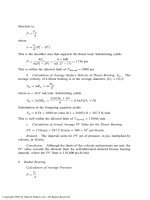
The composite arrangement always reduced the rolling element’s speed. However,
the results are not always completely satisfactory, because the rolling speed is not
low enough. Experiments have indicated that in many cases the rolling speed in
the composite bearing in Fig. 18-2 is too high for a significant improvement in
FIG. 18-5 Ratio of inner race speed to shaft speed vs. shaft speed for the composite
bearing. (From Anderson, Fleming, and Parker, 1972.)
* The U.S. Air Force spends over $20 million annually on replacing rolling-element bearings (Valenti,
1995).
Copyright 2003 by Marcel Dekker, Inc. All Rights Reserved.
fatigue life. Whenever the friction of the rolling-element bearing is much lower
than that of the hydrodynamic journal bearing, the rolling element rotates at
relatively high speed. To improve this combination, a few ideas were suggested to
control the composite bearing and to restrict the rotation of the rolling elements to
a desired speed.
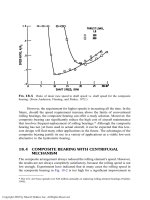
In Fig. 18-6a, a design is shown where the sleeve is connected to a
mechanism similar to a centrifugal clutch; see Harnoy and Rachoor (1993). A
design based on a similar principle was suggested by Silver (1972). A disc with
radial holes is tightly fitted on the sleeve and pins slide along radial holes. Due to
the action of centrifugal force, a friction torque is generated between the pins and
the housing that increases with sleeve speed. This friction torque restricts the

rolling speed and determines the speed of transition from rolling to sliding. The
centrifugal design allows the sleeve to rotate continuously at low speed. This
offers additional advantages, such as enhanced heat transfer from the lubrication
film, (Harnoy and Khonsari, 1996) and improved performance under dynamic
conditions, (Harnoy and Rachoor, 1993). Long life of the rolling element is
maintained because the rolling speed is low. This design has considerable
advantages, in particular for high-speed machinery that involves frequent start-
ups. Figure 18-6b is a design of a composite bearing for radial and thrust loads
with adjustable arrangement.
It is possible to increase the speeds ðo
b
þ o
j
Þ during the transition from
rolling to sliding, resulting in a thicker fluid film at that instant. This can be
achieved by means of a unique design of a delayed centrifugal mechanism where
the motion of the pins is damped as shown in Fig. 18-7. The purpose of this
mechanism is to delay the transition from rolling to sliding during start-up,
resulting in higher speeds ðo
b
þ o
j
Þ at the instant of transition. The delayed
action is advantageous only during the start-up, when the wear is more severe
than that during the stopping period, since a certain time is required to form a
lubricant film or to squeeze it out.
18.4.1 Design for the Desired Rolling Speed
The following derivation is required for the design of a centrifugal mechanism
with the desired rolling speed, o
b

. The derivation is for a short journal bearing
and a typical ball bearing.
The steady rolling speed o
b
can be solved from the friction torque balance,
acting on the sleeve system—a combination of the sleeve and the centrifugal
mechanism. The hydrodynamic torque, M
h
, of a short bearing is:
M
h
¼
LmR
3
C
ðo
j
À o
b
Þ
2p
ð1 Àe
2
Þ
0:5
ð18-3Þ
Here, Rðo
j
À o
b

Þ replaces U in Eq. (7-29).
Copyright 2003 by Marcel Dekker, Inc. All Rights Reserved.
Eq. (18-7); see Fig. 18-4. However, in certain cases, such as in a tightly fitted
conical bearing, the rolling friction is significant and should be considered.
Equation (18-7) yields the following solution for the rolling speed o
b
:
o
b
¼
ðn
2
þ mqÞ
0:5
À n
m
ð18-8Þ
where
m ¼ f
c
m
c
R
m
R
h
ð18-9Þ
n ¼ pLmR
3
Cð1 Àe

2
Þ
0:5
ð18-10Þ
q ¼ 2no
j
ð18-11Þ
The speed o
b
can be determined by selecting the mass of the pins m
c
.
18.5 PERFORMANCE UNDER DYNAMIC
CONDITIONS
The advantages of the composite bearing are quite obvious under steady constant
load. However, the composite bearing did not gain wide acceptance, because
there were concerns about possible adverse effects under unsteady or oscillating
loads (dynamic loads). In rotating machinery, there are always vibrations and the
average load is superimposed by oscillating forces at various frequencies. Harnoy
and Rachoor (1993) analyzed the response of a composite bearing with a
centrifugal mechanism, as shown in Fig. 18-6a and b, under dynamic conditions
of a steady load superimposed with an oscillating load. The analysis involves
angular oscillations of the sleeve, time-variable eccentricity, and unsteady fluid
film pressure.
This analysis is essential for predicting any possible adverse effects of the
composite arrangement on the bearing stability. Most probably, the unstable
region is not identical to that of the common fluid film bearing. Nevertheless,
there are reasons to expect improved performance within the stable region.
The following is an explanation of the criteria for improved bearing
performance under dynamic loads and why composite bearings are expected to

contribute to such an improvement. Unlike operation under steady conditions,
where the journal center is stationary, under dynamic conditions, such as
sinusoidal force, the journal center, O
1
is in continuous motion (trajectory)
relative to the sleeve center O, and the eccentricity e varies with time. For a
periodic load, such as in engines, the journal center O
1
reaches a steady-state
trajectory referred to as journal locus that repeats in each time period. If the
maximum eccentricity e
m
of this locus (the maximum distance O–O
1
in Fig. 18-
1) were to be reduced by the composite arrangement in comparison to the
Copyright 2003 by Marcel Dekker, Inc. All Rights Reserved.
common journal bearing, it would mean that there is an important improvement
in bearing performance. When the eccentricity ratio e ¼ e=C approaches 1, there
is contact and wear of the journal and sleeve surfaces. As discussed in previous
chapters, due to surface roughness, dust, and disturbances, e
m
must be kept low
(relative to 1) to prevent bearing wear.
Of course, one can reduce the maximum eccentricity of the locus by simply
increasing the oil viscosity, m; however, this is undesirable because it will increase
the viscous friction. If it can be shown that a composite bearing can reduce the
maximum eccentricity e
m
, for the same viscosity and dynamic loads, then there is

a potential for energy savings. In that case, it would be possible to reduce the
viscosity and viscous losses without increasing the wear.
There is a simple physical explanation for expecting a significant improve-
ment in the performance of a composite bearing under dynamic conditions,
namely, the relative reduction of e
m
under oscillating loads. Let us consider a
bearing under sinusoidal load. During the cycle period, the critical time is when
the load approaches its peak value. At that instant, the journal center, O
1
is
moving in the radial direction (away from the bearing center O) and the
eccentricity e approaches its maximum value e
m
. At that instant, the fluid film
is squeezed to its minimum thickness.
Under dynamic load, a significant part of the load capacity of the fluid film
is proportional to the sum of the journal and sleeve rotations ðo
b
þ o
j
Þ [see Eq.
(18-1)]. As the external force increases, the fluid film is squeezed and the
hydrodynamic friction torque, M
h
, increases as well, causing the sleeve to rotate
faster (o
b
increases). At that critical instant, the fluid film load capacity increases,
due to a rise in ðo

b
þ o
j
Þ, in the direction directly opposing the journal motion
toward the sleeve surface, resulting in reduced e
m
. The sleeve oscillates
periodically as a pendulum due to the external harmonic load.
However, it will be shown that the complete dynamic behavior is more
complex. The inertia and damping of the sleeve motion cause a phase lag between
the sleeve and the force oscillations. In certain cases, depending on the design
parameters, one can expect adverse effects. If the phase lag becomes excessive, it
would result in unsynchronized sleeve rotation, opposite to the desired direction.
This discussion emphasizes the significance of a full analysis, not only to predict
behavior but also to provide the tools for proper design.
18.5.1 Equations of Motion
The following analysis is for a composite bearing operating at the rated constant
journal speed, with the centrifugal restraint (Fig. 18-6). The length L of the
internal bore of most rolling bearings is short relative to the diameter D. For this
reason, the following is for a short journal bearing, which assumes L ( D. The
analysis can be extended to a finite-length journal bearing; however, it is adequate
Copyright 2003 by Marcel Dekker, Inc. All Rights Reserved.
for our purpose—to compare the dynamic behavior of a composite bearing to that
of a regular one.
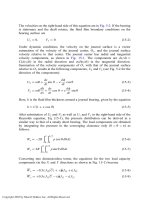
The first step is a derivation of the dynamic equation that describes the
rotation of the composite bearing sleeve unit, consisting of the sleeve, the inner
ring of the rolling bearing, and the centrifugal disc system. The three parts are
tightly fitted and are rotating together at an angular speed o
b
, as shown in Fig.

18-8. This sleeve unit has an equivalent moment of inertia I
eq
. The degree of
freedom of sleeve rotation, which is involved with I
eq
, includes the rolling
elements that rotate at a reduced speed. It is similar to an equivalent moment of
inertia of meshed gears.
A periodic load results in a variable hydrodynamic friction torque, and in
turn there are angular oscillations of the sleeve unit (the angular velocity o
b
varies periodically). The sleeve unit oscillations are superimposed on a constant
FIG. 18-8 Dynamically loaded composite bearing.
Copyright 2003 by Marcel Dekker, Inc. All Rights Reserved.
speed of rotation. At the same time, the mechanical friction between the pins and
the housing damps these oscillations.
The difference between the hydrodynamic (viscous) friction torque M
h
and
the mechanical friction torque of the pins M
f
is the resultant torque that
accelerates the sleeve unit. The rolling friction torque M
r
is small and negligible.
The equation of the sleeve unit motion becomes
M
h
À M
f

¼ I
eq
do
b
dt
ð18-12Þ
Substituting the values of the hydrodynamic torque and the mechanical friction
torque from Eqs. (18-3) and (18-6) into Eq. (18-12) results in the following
equation for the sleeve motion:
LmR
3
C
ðo
j
À o
b
Þ
2p
ð1 Àe
2
Þ
0:5
À m
c
R
m
R
h
o
2

b
f
c
¼ I
eq
do
b
dt
ð18-13Þ
This equation is converted to dimensionless form by dividing all the terms by
I
eq
o
2
j
. The final dimensionless dynamic equation of the sleeve unit motion is
ð1 À xÞH
1
2p
ð1 Àe
2
Þ
0:5
À x
2
H
2
¼
_
xx ð18-14Þ

Here, x is the ratio of the sleeve unit angular velocity to the journal angular
velocity:
x ¼
o
b
o
j
ð18-15Þ
The time derivative
_
xx ¼ dx=d
"
tt is with respect to the dimensionless time,
"
tt ¼ o
j
t,
and the dimensionless parameters H
1
and H
2
are design parameters of the
composite bearing defined by
H
1
¼
LmR
3
CI
eq

o
j
; H
2
¼ m
c
R
m
R
h
f
c
ð18-16Þ
18.5.2 Equation of Journal Motion
Chapter 7 presented the solution of Dubois and Ocvirk (1953) for the pressure
distribution of a short journal bearing under steady conditions. This derivation
was extended in Chapter 15 to a short bearing under dynamic conditions. In this
chapter, this derivation is further extended to a composite bearing where the
sleeve unit rotates at unsteady speed.
It was shown in Chapter 15 that in a journal bearing under dynamic
conditions, the journal center O
1
has an arbitrary velocity described by its two
Copyright 2003 by Marcel Dekker, Inc. All Rights Reserved.
components, de=dt and edf=dt, in the radial and tangential directions, respec-
tively. The purpose of the following analysis is to solve for the journal center
trajectory of a composite bearing.
Let us recall that the Reynolds equation for the pressure distribution p in a
thin incompressible fluid film is
@

@x
h
3
m
@p
@x

þ
@
@z
h
3
m
@p
@z

¼ 6ðU
1
À U
2
Þ
@h
@x
þ 12ðV
2
À V
1
Þð18-17Þ
Similar to the derivation in Sec. 15.2, the journal surface velocity components, U
2

and V
2
are obtained by summing the velocity vector of the surface velocity,
relative to the journal center O
1
(velocity due to journal rotation), and the velocity
vector of O
1
relative to O (velocity due to the motion of the journal center O
1
). At
the same time, the sleeve surface has only tangential velocity, Ro
b
, in the x
direction. In a composite bearing, the fluid film boundary conditions on the right-
hand side of Eq. (18-17) become
V
1
¼ o
j
R
dh
dt
þ
de
dt
cos y þe
df
dt
sin y ð18-18Þ

V
2
¼ 0 ð18-19Þ
U
1
¼ o
b
R ð18-20Þ
U
2
¼ o
j
R þ
de
dt
sin y Àe
df
dt
cos y ð18-21Þ
According to our assumptions, @p=@x on the left-hand side of Eq. (18-17) is
negligible. Considering only the axial pressure gradient and substituting Eqs.
(18-18)–(18-21) into Eq. (18-17) yields
@
@z
h
3
@p
@z

¼ 6m

@
@x
Rðo
j
þ o
b
Þþ6m
de
dt
cos y þe
df
dt
sin y

ð18-22Þ
Integrating Eq. (18-22) twice with the following boundary conditions solves the
pressure wave:
p ¼ 0atz ¼Æ
L
2
ð18-23Þ
Copyright 2003 by Marcel Dekker, Inc. All Rights Reserved.
In the case of a short bearing, the pressure is a function of z and y. The
following are the two equations for the integration of the load capacity
components in the directions of W
x
and W
y
:
W

x
¼À2R
ð
p
0
ð
L=2
0
p cos y dy dz ð18-24Þ
W
y
¼ 2R
ð
p
0
ð
L=2
0
p sin y dy dz ð18-25Þ
The dimensionless load capacity W and the external dynamic load FðtÞ are
defined as follows:
W ¼
C
2
mRo
j
L
3
W ; FðtÞ¼
C

2
mRo
j
L
3
FðtÞð18-26Þ
where the journal speed o
j
is constant. After integration and conversion to
dimensionless form, the following fluid film load capacity components are
obtained:
W
x
¼À
1
2
J
12
eð1 þ xÞþe
_
ffJ
12
þ
_
ee J
22
ð18-27Þ
W
y
¼

1
2
J
11
eð1 þ xÞÀe
_
ffJ
12
À
_
ee J
22
ð18-28Þ
The integrals J
ij
and their solutions are defined according to Eq. (7-13). The
resultant of the load and fluid film force vectors accelerates the journal according
to Newton’s second law:
~
FFðtÞþ
~
WW ¼ m
~
aa ð18-29Þ
Here,
~
aa is the acceleration vector of the journal center O
1
and m is the journal
mass. Dimensionless mass is defined as

m ¼
C
3
o
j
R
L
3
R
2
m ð18-30Þ
After substitution of the acceleration terms in the radial and tangential directions
(directions X and Y in Fig. 18-8) the equations become
F
x
ðtÞÀW
x
¼ m
€
ee À me
_
ff
2
ð18-31Þ
F
y
ðtÞÀW
y
¼Àme
€

ff À 2m
_
ee
_
ff ð18-32Þ
Copyright 2003 by Marcel Dekker, Inc. All Rights Reserved.
Substituting the load capacity components of Eqs. (18-27) and (18-28) into Eqs.
(18-31) and (18-32) yields the final two differential equations of the journal
motion:
FðtÞcosðf ÀpÞ¼À0:5J
12
eð1 þxÞþe
_
ffJ
12
þ
_
ee J
22
þ m
€
ee À me
_
ff
2
ð18-33Þ
FðtÞsinðf ÀpÞ¼0:5J
11
eð1 þxÞÀe
_

ffJ
11
À
_
ee J
12
À me
€
ff À 2m
_
ee
_
ff
ð18-34Þ
Equations (18-33), (18-34), and (18-14) are the three differential equations
required to solve for the three time-dependent functions e; f, and x. These
three variables represent the motion of the shaft center O
1
with time, in polar
coordinates, as well as the rotation of the sleeve unit.
18.5.3 Comparison of Journal Locus under
Dynamic Load
In machinery there are always vibrations and bearing under steady loads are
usually subjected to dynamic oscillating loads. The following is a solution for a
composite bearing under a vertical load consisting of a sinusoidal load super-
imposed on a steady load according to the equation (in this section,
"
FF and
"
mm are

renamed F and m)
FðtÞ¼F
s
þ F
o
sin ao
j
t ð18-35Þ
Here, F
s
is a steady load, F
o
is the amplitude of a sinusoidal force, o is the load
frequency, and a is the ratio of the load frequency to the journal speed:
a ¼
o
o
j
ð18-36Þ
Equations (18-33), (18-34), and (18-14) were solved by finite differences. By
selecting backward differences, the nonlinear terms were linearized. In this way,
the three differential equations were converted to three regular equations. The
finite difference procedure is presented in Sec. 15.4.
Examples of the loci of a composite bearing and a regular journal bearing
are shown in Fig. 18-9 for a ¼ 2 and in Fig. 18-10 for a ¼ 2 and a ¼ 4. Any
reduction in the maximum eccentricity ratio, e
m
, represents a significant improve-
ment in lubrication performance. The curves indicate that the composite bearing
(dotted-line locus) has a lower e

m
than a regular journal bearing (solid-line locus).
An important aspect is that the relative improvement increases whenever e
m
increases (the journal approaches the sleeve surface); thus, the composite bearing
plays an important role in wear reduction. For example, in the heavily loaded
Copyright 2003 by Marcel Dekker, Inc. All Rights Reserved.
bearing in Fig 18-11, the composite bearing nearly doubles the minimum film
thickness e
m
of a regular journal bearing. This can be observed by the distance
between the two loci and the circle e ¼ 1.
If there is a relatively large phase lag between the load and sleeve unit
oscillations, the lubrication performance of the composite bearing can deteriorate.
In order to benefit from the advantages of a composite bearing, in view of the
many design parameters, the designer must in each case conduct a similar
computer simulation to determine the dynamic performance.
18.6 THERMAL EFFECTS
The peak temperature, in the fluid film and on the inner surface of the sleeve (near
the minimum film thickness) was discussed in Sec. 8.6. Excessive peak
temperature T
max
can result in bearing failure, particularly in large bearings
with white metal lining. Therefore, in these cases, it is necessary to limit T
max
during the design stage.
With a properly designed composite bearing, a much more uniform
temperature distribution is expected; since the sleeve unit rotates, the severity
of the peak temperature is reduced.
The heat transfer from the region of the minimum film thickness to the

atmosphere is affected by the rotation of the sleeve as well as many other
parameters, such as bearing materials, lubrication, heat conduction at the contact
between the rolling elements and races, the design of the bearing housing, and its
connection to the body of the machine.
In order to elucidate the effect of the rotation of the sleeve on heat transfer,
Harnoy and Khonsari (1996) studied the effect of sleeve rotation in isolation from
FIG. 18-11 Journal loci of rigid and compliant sleeve bearings under heavy load.
FðtÞ¼800 þ800 sinð2o
j
tÞ. The journal mass is m ¼ 100, H
1
¼ 0:1 and H
2
¼ 100.
Copyright 2003 by Marcel Dekker, Inc. All Rights Reserved.
any other factor that can affect the rate of heat removal from the hydrodynamic oil
film. For this purpose, the heat transfer problem of a hydrodynamic bearing at
steady-state conditions is studied and a comparison made between the tempera-
ture distributions in stationary and rotary sleeves while all other parameters, such
as geometry and materials, are identical for the two cases. For comparison
purposes, a model is presented where the sleeve loses heat to the surroundings at
ambient temperature T
amb
. It has been shown that such a model can yield practical
conclusions concerning the thermal effect of the rotating sleeve in the composite
bearing.
An example of a typical hydrodynamic bearing is selected. The purpose of
the analysis is to determine the temperature distributions inside the rotating and
stationary sleeves. The geometrical parameters and operating conditions of the
two hydrodynamic bearings are summarized in Table 18.1.

18.6.1 The rmal Solution for Sta tionary and
Rotating Sleeves
The temperature distribution in the fluid film is solved by the Reynolds equation,
together with the equation of viscosity variation versus temperature. The viscous
friction losses are dissipated in the fluid as heat, which is transferred by
convection (fluid flow) and conduction through the sleeve. The shaft temperature
TABLE 18-1 Bearing and Lubrication Specifications
Outer sleeve radius, R
o
0.095 m
Shaft radius, R
j
0.05 m
Shaft speed, o
j
3500 RPM
Sleeve wall thickness, b 0.01 m
Sleeve length, L 0.1 m
Sleeve thermal diffusivity, a
b
1:5 Â10
À5
m
2
=s
Sleeve speed, o
b
200 RPM
Clearance, C 0.00006 m
Eccentricity ratio, e 0.5

Length-to-diameter ratio, L=D 1
Thermal conductivity of sleeve material, K
b
45 W=m-K
Density of bush material, r
b
8666 kg=m
3
Specific heat of sleeve material, C
pb
0.343 kJ=kg-K
Thermal conductivity of oil, K
o
0.13 W=m-K
Density of oil, r
o
860 kg=m
3
Ambient temperature, T
amb
24.4

C
Viscosity of the oil at the inlet temperature, m 0.03 kg=m-s
Viscosity–temperature coefficient, b 0.0411=

K
Oil thermal diffusivity, a
o
7.6 Â10

8
m
2
=s
From Harnoy and Khonsari, 1996.
Copyright 2003 by Marcel Dekker, Inc. All Rights Reserved.
is assumed to be constant. The following equation, in a cylindrical coordinate
system ðr; y Þ, was used for solving the temperature distribution in the sleeve (the
coordinate system is fixed to the solid sleeve and rotating with it):
@
2
T
@r
2
þ
1
r
@T
@r
þ
1
r
2
@
2
T
@y
2
¼
1

a
dT
dt
ð18-37Þ
where a is the thermal diffusivity of the solid. For a rotating sleeve in stationary
(Eulerian) coordinates (the sleeve rotates relative to the stationary coordinates)
this equation can be expressed as
@
2
T
@r
2
þ
1
r
@T
@r
þ
1
r
2
@
2
T
@y
2
¼
o
b
a

@T
@y
þ
1
a
dT
dt
ð18-38Þ
where o
b
is the angular speed of the sleeve.
The following order of magnitude analysis intends to show that when the
sleeve rotates above a certain speed, its maximum temperature difference in the
circumferential direction, DT
c
, becomes negligible compared with the maximum
temperature difference, DT
r
, in the radial direction. The order of magnitude of all
terms in Eq. (18-38) are:
@
2
T
@r
2
¼ O
DT
r
b
2


1
r
@T
@r
¼ O
DT
r
R
b
b

1
r
2
@
2
T
@y
2
¼ O
DT
c
pR
2
b

ð18-39aÞ
o
b

a
@T
@y
¼ O
o
b
R
b
a

DT
c
R
b

ð18-39bÞ
Here, b represents the sleeve wall thickness, b ¼ R
o
À R
i
. The radius R is taken as
the average value of the outer and inner radii of the bushing, R
b
¼ðR
o
þ R
i
Þ=2.
Substituting these orders in Eq. (18-38) and assuming b ( R, the order of the
ratio of the temperature gradients is

@T
@r
1
R
@T
@y
¼ O
o
b
R
b
b
a
b

ð18-40Þ
The dimensionless parameter on the right-hand side of Eq. (18-40) is a modified
Peclet number (Pe). Equation (18-40) indicates that when Pe ) 1, the radial
temperature gradient is much higher than the temperature gradient in the
circumferential direction, and the temperature distribution can be assumed to
Copyright 2003 by Marcel Dekker, Inc. All Rights Reserved.
be uniform around the sleeve. In fact, in the circumferential direction, most of the
heat is effectively transferred by the moving mass of the rotating sleeve and only a
negligible amount of heat is transferred by conduction. In the example (Table
18-1), if the sleeve speed is 200 RPM, the Peclet number is
Pe ¼
o
b
R
b

b
a
b
¼ 692 ð18-41Þ
This number indicates that the circumferential temperature gradient is relatively
low, and only heat conduction in the radial direction needs to be considered in
solving for the temperature distribution. It is interesting to note that there would
be no significant change in the composite bearing thermal characteristics even at
much lower sleeve speeds. For example, for o
b
¼30 RPM, the resulting Pe is
above 100, and the assumption of negligible circumferential temperature gradi-
ents should still hold. It should be noted that a composite bearing design
operating at a low sleeve speed might not be desirable. Elastohydrodynamic
lubrication in the rolling bearing requires a certain minimum speed below which
FIG. 18-12 Thermohydrodynamic solution showing the isotherm contours plot in a
stationary sleeve of a journal bearing. L=D ¼ 1, e ¼ 0:5, N
shaft
¼ 3500 RPM. (From
Harnoy and Khonsari, 1996.)
Copyright 2003 by Marcel Dekker, Inc. All Rights Reserved.
the friction is somewhat higher, as the rolling bearing friction–velocity curve
presented in Fig. 18-4 demonstrates.
A full thermohydrodynamic analysis was performed with the bearing
specifications listed in Table 18-1 assuming a stationary sleeve. The solution
for the temperature profile in the stationary sleeve is presented by isotherms in
Fig. 18-12.
Hydrodynamic lubrication theory indicates that the amount of heat dissi-
pated in the oil film is proportional to the average shear rate and, in turn,
proportional to the difference between the journal and sleeve speeds ðo

j
À o
b
Þ.
Therefore, it is reasonable to assume that the heat flux from the oil film to the
surroundings is also proportional to ðo
j
À o
b
Þ. Therefore, the ratio of the radial
heat fluxes of rotating and stationary is
Q
rotating sleeve
¼ Q
rigid sleeve
ðo
j
À o
b
Þ
o
j
ð18-42Þ
FIG. 18-13 Isotherm contours plot of a rotating sleeve unit. (From Harnoy and
Khonsari, 1996.)
Copyright 2003 by Marcel Dekker, Inc. All Rights Reserved.
The surface temperatures T
i
(inner wall) and T
o

(outside wall) of the sleeve are
solved by the following equations:
T
i
¼ T
amb
þ Q
rotating sleeve
lnðR
o
=R
i
Þ
2pk
b
L
þ
1
2pR
o
Lh
&'
ð18-43Þ
T
o
¼ T
i
À Q
rotating sleeve
lnðR

o
=R
i
Þ
2pk
b
L
&'
ð18-44Þ
Here, h is the correction coefficient. The temperature distribution in the sleeve is
obtained from
T ÀT
i
T
o
À T
i
¼
lnðr=R
i
Þ
lnðR
o
=R
i
Þ
ð18:45Þ
The results are circular isotherms, as shown in Fig. 18-13. The uniformity in the
temperature profile, together with a reduction in the maximum temperature
(59.7


C for composite bearing versus 71

C for a conventional hydrodynamic
bearing), is indicative of the superior thermal performance.
Copyright 2003 by Marcel Dekker, Inc. All Rights Reserved.
19
Non-Newtonian Viscoelastic E¡ects
19.1 INTRODUCTION
The previous chapters focused on Newtonian lubricants such as regular mineral
oils. However, non-Newtonian multigrade lubricants, also referred to as VI
(viscosity index) improved oils are in common use today, particularly in motor
vehicle engines. The multigrade lubricants include additives of long-chain
polymer molecules that modify the flow characteristics of the base oils. In this
chapter, the hydrodynamic analysis is extended for multigrade oils.
The initial motivation behind the development of the multigrade lubricants
was to reduce the dependence of lubricant viscosity on temperature (to improve
the viscosity index). This property is important in motor vehicle engines, e.g.,
starting the engine on cold mornings. Later, experiments indicated that multi-
grade lubricants have complex non-Newtonian characteristics. The polymer-
containing lubricants were found to have other rheological properties in addition
to the viscosity. These lubricants are viscoelastic fluids, in the sense that they have
viscous as well as elastic properties.
Polymer additives modify several flow characteristics of the base oil.
1. The polymer additives increase the viscosity of the base oil.
2. The polymer additives moderate the reduction of viscosity with
temperature (improve the viscosity index).
Copyright 2003 by Marcel Dekker, Inc. All Rights Reserved.
3. The viscosity becomes a decreasing function of shear rate (shear-
thinning property).

4. Normal stresses are introduced. In simple shear flow, u ¼ uðyÞ, there
are normal stress differences s
x
À s
y
(first difference) and s
y
À s
z
(second difference). The first difference is much higher than the second
difference.
5. The polymer additives introduce stress-relaxation characteristics into
the fluid, exemplified by a phase lag between the shear stress and a
periodic shear rate. This property is what is meant by the term
viscoelasticity; namely, the fluid becomes elastic as well as viscous.
Although multi grade oils were developed to improve the viscosity index,
later experiments revealed a significant improvement in the lubrication perfor-
mance of journal bearings that cannot be explained by changes of viscosity.
Dubois et al. (1960) compared the performance of mineral oils and VI improved
oils in journal bearings under static load. They used high journal speeds and
measured load capacity, friction and eccentricity. The results indicated a superior
performance of the multigrade oils with polymer additives. Additional conclusion
of this investigation (important for comparison with analytical investigations) is
that the relative improvement in load capacity of the VI improved oils becomes
greater as the eccentricity increases. Okrent (1961) and Savage and Bowman
(1961) found less friction and wear in the connecting-rod bearing in a car engine
(dynamically loaded journal bearing).
Analytical investigations showed that the improvements in the lubrication
performance of VI improved oils are not due to changes in the viscosity. Horowitz
and Steidler (1960) performed analytical investigation and showed that the

improvement in the lubrication performance could not be accounted for by the
different function of viscosity versus shear rate and temperature. In fact, they
found that the non-Newtonian viscosity increases the friction coefficient (opposite
trend to the experiments of Dubois et al., 1960).
A survey of the previous analytical investigation by Harnoy (1978) shows
that the measured order of magnitude of the first and second normal stresses is
too low to explain any significant improvement in the lubrication performance.
This discussion indicates that the elasticity of the fluid (stress-relaxation effect) is
the most probable explanation of the improvement in performance of viscoelastic
lubricants.
The criterion for improvement of the lubrication performance is very
important. For example, polymer additives increase the viscosity of mineral
oils; in turn, the load capacity increases. However, our basis of comparison is the
load capacity at equivalent viscosity and bearing geometry. Higher viscosity on
its own is not considered as an improvement in the lubrication performance,
because the friction losses as well as load capacity are both proportional to the
Copyright 2003 by Marcel Dekker, Inc. All Rights Reserved.