Bearing Design in Machinery Episode 1 Part 8 ppt

The journal surface velocity is U ¼ Ro
j
, and the sleeve surface velocity is the
product xU, where x is the rolling-to-sliding ratio. The common journal bearing
has a pure sliding and x ¼ 0, while in pure rolling, x ¼ 1. For all other
combinations, 0 < x < 1.
The tangential velocities (in the x direction) of the fluid–film boundaries of
the two surfaces are
U
1
¼ R
1
o
b
¼ xRo
j
U
2
¼ Ro
j
cos a % Ro
j
ð6-18Þ
The normal components, in the y direction, of the velocity of the fluid film
boundaries (journal and sleeve surfaces) are
V
1
¼ 0
V
2
¼ Ro

j
@h
@x
ð6-19Þ
For the general case of a combined rolling and sliding, the expression on the
right-hand side of Reynolds equation is obtained by substituting the preceding
components of the surface velocity:
6ðU
1
À U
2
Þ
@h
@x
þ 12ðV
2
À V
1
Þ¼6ðxU À U Þ
@h
@x
þ 12ðU
@h
@x
À 0Þ
¼ 6Uð1 þxÞ
@h
@x
ð6-20Þ
Here, U ¼ Ro

j
is the journal surface velocity. Finally, the Reynolds equation for
a combined rolling and sliding of a journal bearing is as follows:
@
@x
h
3
m
@p
@x

þ
@
@z
h
3
m
@p
@z

¼ 6Ro
j
ð1 þxÞ
@h
@x
ð6-21aÞ
For x ¼ 0 and x ¼ 1, the right-hand-side of the Reynolds equation is in
agreement with the previous derivations for pure sliding and pure rolling,
respectively. The right-hand side of Eq. (6-21a) indicates that pure rolling
action doubles the pressure wave in comparison to a pure sliding.

Equation (6-21a) is often written in the basic form:
@
@x
h
3
m
@p
@x

þ
@
@z
h
3
m
@p
@z

¼ 6Rðo
j
þ o
b
Þ
@h
@x
ð6-21bÞ
In journal bearings, the difference between the journal radius and the bearing
radius is small and we can assume that R
1
% R.

Copyright 2003 by Marcel Dekker, Inc. All Rights Reserved.
6.5 PRESSURE WAVE IN A LONG JOURNAL
BEARING
For a common long journal bearing with a stationary sleeve, the pressure wave is
derived by a double integration of Eq. (6.12). After the first integration, the
following explicit expression for the pressure gradient is obtained:
dp
dx
¼ 6Um
h þ C
1
h
3
ð6-22Þ
Here, C
1
is a constant of integration. In this equation, a regular derivative replaces
the partial one, because in a long bearing, the pressure is a function of one
variable, x, only. The constant, C
1
, can be replaced by h
0
, which is the film
thickness at the point of peak pressure. At the point of peak pressure,
dp
dx
¼ 0ath ¼ h
0
ð6-23Þ
Substituting condition (6-23), in Eq. (6-22) results in C

1
¼Àh
0
, and Eq. (6-22)
becomes
dp
dx
¼ 6Um
h À h
0
h
3
ð6-24Þ
Equation (6-24) has one unknown, h
0
, which is determined later from additional
information about the pressure wave.
The expression for the pressure distribution (pressure wave) around a
journal bearing, along the x direction, is derived by integration of Eq. (6-24),
and there will be an additional unknown—the constant of integration. By using
the two boundary conditions of the pressure wave, we solve the two unknowns,
h
0
, and the second integration constant.
The pressures at the start and at the end of the pressure wave are usually
used as boundary conditions. However, in certain cases the locations of the start
and the end of the pressure wave are not obvious. For example, the fluid film of a
practical journal bearing involves a fluid cavitation, and other boundary condi-
tions of the pressure wave are used for solving the two unknowns. These
boundary conditions are discussed in this chapter. The solution method of two

unknowns for these boundary conditions is more complex and requires computer
iterations.
Replacing x by an angular coordinate y, we get
x ¼ Ry ð6-25Þ
Copyright 2003 by Marcel Dekker, Inc. All Rights Reserved.
Equation (6-24) takes the form
dp
dy
¼ 6URm
h À h
0
h
3
ð6-26Þ
For the integration of Eq. (6-26), the boundary condition at the start of the
pressure wave is required. The pressure wave starts at y ¼ 0, and the magnitude
of pressure at y ¼ 0isp
0
. The pressure, p
0
, can be very close to atmospheric
pressure, or much higher if the oil is fed into the journal bearing by an external
pump.
The film thickness, h, as a function of y for a journal bearing is given in Eq.
(6-3), hðyÞ¼Cð1 þe cos yÞ. After substitution of this expression into Eq. (6-26),
the pressure wave is given by
C
2
6mUR
ðp Àp

0
Þ¼
ð
y
0
dy
ð1 þecos yÞ
2
À
h
0
C
ð
y
0
dy
ð1 þecos yÞ
3
ð6-27Þ
The pressure, p
0
, is determined by the oil supply pressure (inlet pressure). In a
common journal bearing, the oil is supplied through a hole in the sleeve, at y ¼ 0.
The oil can be supplied by gravitation from an oil container or by a high-pressure
pump. In the first case, p
0
is only slightly above atmospheric pressure and can be
approximated as p
0
¼ 0. However, if an external pump supplies the oil, the pump

pressure (at the bearing inlet point) determines the value of p
0
. In industry, there
are often central oil circulation systems that provide oil under pressure for the
lubrication of many bearings.
The two integrals on the right-hand side of Eq. (6-27) are functions of the
eccentricity ratio, e. These integrals can be solved by numerical or analytical
integration. Sommerfeld (1904) analytically solved these integrals for a full
(360

) journal bearing. Analytical solutions of these two integrals are included in
integral tables of most calculus textbooks. For a full bearing, it is possible to solve
for the load capacity even in cases where p
0
can’t be determined. This is because
p
0
is an extra constant hydrostatic pressure around the bearing, and, similar to
atmospheric pressure, it does not contribute to the load capacity.
In a journal bearing, the pressure that is predicted by integrating Eq. (6-27)
increases (above the inlet pressure, p
0
) in the region of converging clearance,
0 < y < p. However, in the region of a diverging clearance, p < y < 2p, the
pressure wave reduces below p
0
. If the oil is fed at atmospheric pressure, the
pressure wave that is predicted by integration of Eq. (6-27) is negative in the
divergent region, p < y < 2p. This analytical solution is not always valid,
because a negative pressure would result in a ‘‘fluid cavitation.’’ The analysis

may predict negative pressures below the absolute zero pressure, and that, of
course, is physically impossible.
Copyright 2003 by Marcel Dekker, Inc. All Rights Reserved.
A continuous fluid film cannot be maintained at low negative pressure
(relative to the atmospheric pressure) due to fluid cavitation. This effect occurs
whenever the pressure reduces below the vapor pressure of the oil, resulting in an
oil film rupture. At low pressures, the boiling process can take place at room
temperature; this phenomenon is referred to as fluid cavitation. Moreover, at low
pressure, the oil releases its dissolved air, and the oil foams in many tiny air
bubbles. Antifoaming agents are usually added into the oil to minimize this effect.
As a result of cavitation and foaming, the fluid is not continuous in the
divergent clearance region, and the actual pressure wave cannot be predicted
anymore by Eq. (6-27). In fact, the pressure wave is maintained only in the
converging region, while the pressure in most of the diverging region is close to
ambient pressure. Cole and Hughes (1956) conducted experiments using a
transparent sleeve. Their photographs show clearly that in the divergent region,
the fluid film ruptures into filaments separated by air and lubricant vapor.
Under light loads or if the supply pressure, p
0
, is high, the minimum
predicted pressure in the divergent clearance region is not low enough to generate
a fluid cavitation. In such cases, Eq. (6-27) can be applied around the complete
journal bearing. The following solution referred to as the Sommerfeld solution,is
limited to cases where there is a full fluid film around the bearing.
6.6 SOMMERFELD SOLUTION OF THE
PRESSURE WAVE
Sommerfeld (1904) solved Eq. (6-27) for the pressure wave and load capacity of a
full hydrodynamic journal bearing (360

) where a fluid film is maintained around

the bearing without any cavitation. This example is of a special interest because
this was the first analytical solution of a hydrodynamic journal bearing based on
the Reynolds equation. In practice, a full hydrodynamic lubrication around the
bearing is maintained whenever at least one of the following two conditions are
met:
a. The feed pressure, p
0
, (from an external oil pump), into the bearing is
quite high in order to maintain positive pressures around the bearing
and thus prevent cavitation.
b. The journal bearing is lightly loaded. In this case, the minimum
pressure is above the critical value of cavitation.
Sommerfeld assumed a periodic pressure wave around the bearing; namely, the
pressure is the same at y ¼ 0 and y ¼ 2p:
p
ðy¼0Þ
¼ p
ðy¼2pÞ
ð6-28Þ
Copyright 2003 by Marcel Dekker, Inc. All Rights Reserved.
The unknown, h
0
, that represents the film thickness at the point of a peak pressure
can be solved from Eq. (6-27) and the Sommerfeld boundary condition in Eq.
(6-28). After substituting p Àp
0
¼ 0, at y ¼ 2p, Eq. (6-27) yields
ð
2p
0

dy
ð1 þ e cos yÞ
2
À
h
0
C
ð
2p
0
dy
ð1 þecos yÞ
3
¼ 0 ð6-29Þ
This equation can be solved for the unknown, h
0
. The following substitutions for
the values of the integrals can simplify the analysis of hydrodynamic journal
bearings:
J
n
¼
ð
2p
0
dy
ð1 þ e cos yÞ
n
ð6-30Þ
I

n
¼
ð
2p
0
cos y dy
ð1 þecos yÞ
n
ð6-31Þ
Equation (6-29) is solved for the unknown, h
0
, in terms of the integrals J
n
:
h
0
C
¼
J
2
J
3
ð6-32Þ
Here, the solutions for the integrals J
n
are:
J
1
¼
2p

ð1 Àe
2
Þ
1=2
ð6-33Þ
J
2
¼
2p
ð1 Àe
2
Þ
3=2
ð6-34Þ
J
3
¼ 1 þ
1
2
e
2

2p
ð1 Àe
2
Þ
5=2
ð6-35Þ
J
4

¼ 1 þ
3
2
e
2

2p
ð1 Àe
2
Þ
7=2
ð6-36Þ
The solutions of the integrals I
n
are required later for the derivation of the
expression for the load capacity. The integrals I
n
can be obtained from J
n
by the
following equation:
I
n
¼
J
nÀ1
À J
n
e
ð6-37Þ

Sommerfeld solved for the integrals in Eq. (6-27), and obtained the following
equation for the pressure wave around an infinitely long journal bearing with a
full film around the journal bearing:
p À p
0
¼
6mUR
C
2
eð2 þecos yÞsin y
ð2 þe
2
Þð1 þ e cos yÞ
2
ð6-38Þ
Copyright 2003 by Marcel Dekker, Inc. All Rights Reserved.
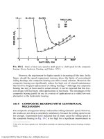
The curves in Fig. 6-4 are dimensionless pressure waves, relative to the
inlet pressure, for various eccentricity ratios, e. The pressure wave is an
antisymmetrical function on both sides of y ¼ p. The curves indicate that the
peak pressure considerably increases with the eccentricity ratio, e. According to
Eq. (6-38), the peak pressure approaches infinity when e approaches 1. However,
this is not possible in practice because the surface asperities prevent a complete
contact between the sliding surfaces.
6.7 JOURNAL BEARING LOAD CAPACITY
Figure 6-5 shows the load capacity, W , of a journal bearing and its two
components, W
x
and W
y
. The direction of W

x
is along the bearing symmetry
line O
O
1
. This direction is inclined at an attitude angle, f, from the direction of
the external force and load capacity, W . In Fig. 6-5 the external force is in a
vertical direction. The direction of the second component, W
y
is normal to the W
x
direction.
The elementary load capacity, dW, acts in the direction normal to the
journal surface. It is the product of the fluid pressure, p, and an elementary area,
FIG. 6-4 Pressure waves in an infinitely long, full bearing according to the Sommerfeld
solution.
Copyright 2003 by Marcel Dekker, Inc. All Rights Reserved.
The two components of the load capacity, W
x
and W
y
, are in the X and
Y directions, respectively, as indicated in Fig. 6-5. Note the negative sign in
Eq. (6-40), since dW
x
is opposite to the W
x
direction. The load components are:
W
x

¼ÀLR
ð
2p
0
p cos y dy ð6-42Þ
W
y
¼ LR
ð
2p
0
p sin y dy ð6-43Þ
The attitude angle f in Fig. 6-5 is determined by the ratio of the force
components:
tan f ¼
W
y
W
x
ð6-44Þ
6.8 LOAD CAPACITY BASED ON SOMMERFELD
CONDITIONS
The load capacity components can be solved by integration of Eqs. (6-42 and
(6-43), where p is substituted from Eq. (6-38). However, the derivation can be
simplified if the load capacity components are derived directly from the basic Eq.
(6-24) of the pressure gradient. In this way, there is no need to integrate the
complex Eq. (6-38) of the pressure wave. This can be accomplished by employing
the following identity for product derivation:
ðuvÞ
0

¼ uv
0
þ vu
0
ð6-45Þ
Integrating and rearranging Eq. (6-45) results in
ð
uv
0
¼ uv À
ð
u
0
v ð6-46Þ
In order to simplify the integration of Eq. (6-42) for the load capacity component
W
x
, the substitutions u ¼ p and v
0
¼ cos y are made. This substitution allows the
use of the product rule in Eq. (6-46), and the integral in Eq. (6-42) results in the
following terms:
ð
p cos y dy ¼ p sin y À
ð
dp
dy
sin y dy ð6-47Þ
In a similar way, for the load capacity component, W
y

, in Eq. (6-43), the
substitutions u ¼ p and v
0
¼ sin y result in
ð
p sin y dy ¼Àp cos y þ
ð
dp
dy
cos y dy ð6-48Þ
Copyright 2003 by Marcel Dekker, Inc. All Rights Reserved.
Equations (6-47) and (6-48) indicate that the load capacity components in Eqs.
(6-42) and (6-43) can be solved directly from the pressure gradient. By using this
method, it is not necessary to solve for the pressure wave in order to find the load
capacity components (it offers the considerable simplification of one simple
integration instead of a complex double integration). The first term, on the right-
hand side in Eqs. (6-47) and (6-48) is zero, when integrated around a full bearing,
because the pressure, p, is the same at y ¼ 0 and y ¼ 2p.
Integration of the last term in Eq. (6-47), in the boundaries y ¼ 0and
y ¼ 2p, indicates that the load component, W
x
, is zero. This is because it is an
integration of the antisymmetrical function around the bearing (the function is
antisymmetric on the two sides of the centerline O
O
1
, which cancel each other).
Therefore:
W
x

¼ 0 ð6-49Þ
Integration of Eq. (6-43) with the aid of identity (6-48), and using the value of h
0
in Eq. 6-32 results in
W
y
¼
6mUR
2
L
C
2
I
2
À
J
2
J
3
I
3

ð6-50Þ
Substituting for the values of I
n
and J
n
as a function of e yields the following
expression for the load capacity component, W
y

. The other component is W
x
¼ 0;
therefore, for the Sommerfeld conditions, W
y
is equal to the total load capacity,
W ¼ W
y
:
W ¼
12pmUR
2
L
C
2
e
ð2 þe
2
Þð1 À e
2
Þ
1=2
ð6-51Þ
The attitude angle, f, is derived from Eq. (6-44). For Sommerfeld’s conditions,
W
x
¼ 0 and tan f !1; therefore,
f ¼
p
2

ð6-52Þ
Equation (6-52) indicates that in this case, the symmetry line O
O
1
is normal to
the direction of the load capacity W.
6.9 FRICTION IN A LONG JOURNAL BEARING
The bearing friction force, F
f
, is the viscous resistance force to the rotation of the
journal due to high shear rates in the fluid film. This force is acting in the
tangential direction of the journal surface and results in a resistance torque to the
Copyright 2003 by Marcel Dekker, Inc. All Rights Reserved.
rotation of the journal. The friction force is defined as the ratio of the friction
torque, T
f
, to the journal radius, R:
F
f
¼
T
f
R
ð6-53Þ
The force is derived by integration of the shear stresses over the area of the
journal surface, at y ¼ h, around the bearing. The shear stress distribution at the
journal surface (shear at the wall, t
w
) around the bearing, is derived from the
velocity gradient, as follows:

t
w
¼ m
du
dy




ðy¼hÞ
ð6-54Þ
The friction force is obtained by integration:
F
f
¼
ð
A
t
ðy¼hÞ
dA ð6-55Þ
After substituting dA ¼ RL dy in Eq. (6-55), the friction force becomes
F
f
¼ mRL
ð
2p
0
t
ðy¼hÞ
dy ð6-56Þ

Substitution of the value of the shear stress, Eq. (6-56) becomes
F
f
¼ mURL
ð
2p
0
4
h
À
3h
0
h
2

dy ð6-57Þ
If we apply the integral definitions in Eq. (6-30), the expression for the friction
force becomes
F
f
¼
mRL
C
4 J
1
À 3
J
2
2
J

3

ð6-58Þ
The integrals J
n
are functions of the eccentricity ratio. Substituting the solution of
the integrals, J
n
, in Eqs. (6.33) to (6.37) results in the following expression for the
friction force:
F
f
¼
mURL
C
4pð1 þ2e
2
Þ
ð2 þe
2
Þð1 À e
2
Þ
1=2
ð6-59Þ
Let us recall that the bearing friction coefficient, f , is defined as
f ¼
F
f
W

ð6-60Þ
Copyright 2003 by Marcel Dekker, Inc. All Rights Reserved.
Substitution of the values of the friction force and load in Eq. (6-60) results in a
relatively simple expression for the coefficient of friction of a long hydrodynamic
journal bearing:
f ¼
C
R
1 þ 2e
2
3e
ð6-61Þ
Comment: The preceding equation for the friction force in the fluid film is based
on the shear at y ¼ h. The viscous friction force around the bearing bore surface,
at y ¼ 0, is not equal to that around the journal surface, at y ¼ h. The viscous
friction torque on the journal surface is unequal to that on the bore surface
because the external load is eccentric to the bore center, and it is an additional
torque. However, the friction torque on the journal surface is the actual total
resistance to the journal rotation, and it is used for calculating the friction energy
losses in the bearing.
6.10 POWER LOSS ON VISCOUS FRICTION
The energy loss, per unit of time (power loss)
_
EE
f
, is determined from the friction
torque, or friction force, by the following equations:
_
EE
f

¼ T
f
o ¼ F
f
U ð6-62Þ
where o ðrad=sÞ is the angular velocity of the journal. Substituting Eq. (6-59) into
Eq. (6-62) yields
_
EE
f
¼
mU
2
RL
C
4pð1 þ2e
2
Þ
ð2 þe
2
Þð1 Àe
2
Þ
1=2
ð6-63Þ
The friction energy losses are dissipated in the lubricant as heat. Knowledge of
the amount of friction energy that is dissipated in the bearing is very important for
ensuring that the lubricant does not overheat. The heat must be transferred from
the bearing by adequate circulation of lubricant through the bearing as well as by
conduction of heat from the fluid film through the sleeve and journal.

6.11 SOMMERFELD NUMBER
Equation (6-51) is the expression for the bearing load capacity in a long bearing
operating at steady conditions with the Sommerfeld boundary conditions for the
pressure wave. This result was obtained for a full film bearing without any
cavitation around the bearing. In most practical cases, this is not a realistic
expression for the load capacity, since there is fluid cavitation in the diverging
clearance region of negative pressure. The Sommerfeld solution for the load
capacity has been improved by applying a more accurate analysis with realistic
Copyright 2003 by Marcel Dekker, Inc. All Rights Reserved.
boundary conditions of the pressure wave. This solution requires iterations
performed with the aid of a computer.
In order to simplify the design of hydrodynamic journal bearings, the
realistic results for the load capacity are provided in dimensionless form in tables
or graphs. For this purpose, a widely used dimensionless number is the
Sommerfeld number, S.
Equation (6-51) can be converted to dimensionless form if all the variables
with dimensions are placed on the left-hand side of the equations and the
dimensionless function of e on the right-hand side. Also, it is the tradition in
this discipline to have the Sommerfeld dimensionless group as a function of
journal speed, n, in revolutions per second, and the average bearing pressure, P,
according to the following substitutions:
U ¼ 2pRn ð6-64Þ
W ¼ 2RLP ð6-65Þ
By substituting Eqs. (6.64) and (6.65) into Eq. (6.51), we obtain the following
dimensionless form of the Sommerfeld number for an infinitely long journal
bearing where cavitation is disregarded:
S ¼
mn
P
R

C

2
¼
ð2 þ e
2
Þð1 À e
2
Þ
1=2
12p
2
e
ð6-66Þ
The dimensionless Sommerfeld number is a function of e only. For an infinitely
long bearing and the Sommerfeld boundary conditions, the number S can be
calculated via Eq. (6-66). However, for design purposes, we use the realistic
conditions for the pressure wave. The values of S for various ratios of length and
diameter, L=D, have been computed; the results are available in Chapter 8 in the
form of graphs and tables for design purposes.
6.12 PRACTICAL PRESSURE BOUNDARY
CONDITIONS
The previous discussion indicates that for most practical applications in machin-
ery the pressures are very high and cavitation occurs in the diverging region of the
clearance. For such cases, the Sommerfeld boundary conditions do not apply and
the pressure distribution can be solved for more realistic conditions. In an actual
journal bearing, there is no full pressure wave around the complete bearing, and
there is a positive pressure wave between y
1
and y

2
. Outside this region, there is
cavitation and low negative pressure that can be ignored for the purpose of
calculating the load capacity. The value of y
2
is unknown, and an additional
condition must be applied for the solution. The boundary condition commonly
used is that the pressure gradient is zero at the end of the pressure wave, at y
2
.
Copyright 2003 by Marcel Dekker, Inc. All Rights Reserved.
This is equivalent to the assumption that there is no flow, u, in the x direction at
y
2
. When the lubricant is supplied at y
1
at a pressure p
0
, the following boundary
conditions can be applied:
p ¼ p
0
at y ¼ y
1
dp
dy
¼ 0aty ¼ y
2
ð6-67Þ
p ¼ 0aty ¼ y

2
In most cases, the feed pressure is close to ambient pressure at y ¼ 0, and the first
boundary condition is p ¼ 0aty ¼ 0. The pressure wave with the foregoing
boundary conditions is shown in Fig. 6-6.
The location of the end of the pressure wave, y
2
, is solved by iterations. The
solution is performed by guessing a value for y
2
that is larger then 180

, then
integrating Eq. (6-27) at the boundaries from 0 to y
2
. The solution is obtained
when the pressure at y
2
is very close to zero.
Figure 6-6 indicates that the angle y
2
and the angle of the peak pressure are
symmetrical on both sides of y ¼ p; therefore both have an equal film thickness h
(or clearance thickness). The constant, h
0
, representing the film thickness at the
maximum pressure is
h
0
¼ Cð1 þcos y
2

Þð6-68Þ
After the integration is completed, the previous guess for y
2
is corrected until a
satisfactory solution is obtained (the pressure at y
2
is very close to zero).
Preparation of a small computer program to solve for y
2
by iterations is
recommended as a beneficial exercise for the reader. After h
0
is solved the
pressure wave can be plotted.
FIG. 6-6 Pressure wave plot under realistic boundary conditions.
Copyright 2003 by Marcel Dekker, Inc. All Rights Reserved.
Example Problem 6-1
Ice Sled
Two smooth cylindrical sections support a sled as shown in Fig. 6-7. The sled is
running over ice on a thin layer of water film. The total load (weight of the sled
and the person) is 1000 N. This load is acting at equal distances between the two
blades. The sled velocity is 15 km=h, the radius of the blade is 30 cm, and its
width is L ¼ 90 cm. The viscosity of water m ¼ 1:792 Â10
À3
N-s=m
2
.
a. Find the pressure distribution at the entrance region of the fluid film
under the ski blade as it runs over the ice. Derive and plot the pressure
wave in dimensionless form.

b. Find the expression for the load capacity of one blade.
c. Find the minimum film thickness ðh
n
¼ h
min
Þ of the thin water layer.
Solution
a. Pressure Distribution and Pressure Wave
For h
n
=R ( 1, the pressure wave is generated only near the minimum-film
region, where x ( R,orx=R ( 1.
For a small value of x=R, the equation for the clearance, between the
quarter-cylinder and the ice, h ¼ hðxÞ, can be approximated by a parabolic wedge.
The following expression is obtained by expanding the equation for the variable
clearance, hðxÞ, which is equal to the fluid-film thickness, into a Taylor series and
truncating powers higher than x
2
(see Chapter 4).
If the minimum thickness of the film is h
n
¼ h
min
, the equation for the
variable clearance becomes
hðxÞ¼h
n
þ
x
2

2R
FIG. 6-7 Sled made of two quarter-cylinder.
Copyright 2003 by Marcel Dekker, Inc. All Rights Reserved.
For dimensionless analysis, the clearance function is written as
hðxÞ¼h
n
1 þ
x
2
2Rh
n

The width, L (in the direction normal to the sled speed), is very large in
comparison to the film length in the x direction. Therefore, it can be considered
an infinitely long bearing, and the pressure gradient is
dp
dx
¼ 6mU
h À h
0
h
3
The unknown, h
0
, is the fluid film thickness at the point of peak pressure, where
dp=dx ¼ 0.
Conversion to Dimensionless Terms. The conversion to dimensionless
terms is similar to that presented in Chapter 4. The length, x, is normalized by
ffiffiffiffiffiffiffiffiffiffi
2Rh

n
p
, and the dimensionless terms are defined as
"
xx ¼
x
ffiffiffiffiffiffiffiffiffiffi
2Rh
n
p
and
"
hh ¼
h
h
n
The dimensionless clearance gets a simple form:
"
hhð
"
xxÞ¼1 þ
"
xx
2
Using the preceding substitutions, the pressure gradient equation takes the form
dp
dx
¼
6mU
h

2
n
"
hh À
"
hh
0
ð1 þ
"
xx
2
Þ
3
Here the unknown, h
0
, is replaced by
"
hh
0
¼ 1 þ
"
xx
2
0
The unknown, h
0
, is replaced by unknown x
0
, which describes the location of the
peak pressure. Using the foregoing substitutions, the pressure gradient equation is

reduced to
dp
dx
¼
6mU
h
2
n
"
xx
2
À
"
xx
2
0
ð1 þ
"
xx
2
Þ
3
Converting dx into dimensionless form produces
dx ¼
ffiffiffiffiffiffiffiffiffiffi
2Rh
n
p
d
"

xx
The dimensionless differential equation for the pressure takes the form
h
2
n
ffiffiffiffiffiffiffiffiffiffi
2Rh
n
p
6mU
dp ¼
"
xx
2
À
"
xx
2
0
ð1 þ
"
xx
2
Þ
3
d
"
xx
Copyright 2003 by Marcel Dekker, Inc. All Rights Reserved.
Here, the dimensionless pressure is

"
pp ¼
h
2
n
6Um
ffiffiffiffiffiffiffiffiffiffi
2Rh
n
p
p
The final equation for integration of the dimensionless pressure is
"
pp ¼
h
2
n
ffiffiffiffiffiffiffiffiffiffi
2Rh
n
p
1
6mU
ð
p
0
dp ¼
ð
x
1

"
xx
2
À
"
xx
2
0
ð1 þ
"
xx
2
Þ
3
d
"
xx þ p
0
Here p
0
is a constant of integration, which is atmospheric pressure far from the
minimum clearance. In this equation, p
0
and x
0
are two unknowns that can be
solved for by the following boundary conditions of the pressure wave:
at x ¼1; p ¼ 0
at x ¼ 0; p ¼ 0
The first boundary condition, p ¼ 0atx ¼1, yields p

0
¼ 0. The second
unknown, x
0
, is solved for by iterations (trial and error). The value of x
0
is
varied until the second boundary condition of the pressure wave, p ¼ 0atx ¼ 0,
is satisfied.
Numerical Solution by Iterations. For numerical integration, the boundary
"
xx ¼1is replaced by a relatively large finite dimensionless value where pressure
is small and can be disregarded, such as
"
xx ¼ 4.
The numerical solution involves iterations for solving for x
0
. Each one of
the iterations involves integration in the boundaries from 4 to 0. The solution for
x
0
is obtained when the pressure at x ¼ 0 is sufficiently close to zero. Using trial
and error, we select each time a value for x
0
and integrate. This is repeated until
the value of the dimensionless pressure is nearly zero at x ¼ 0. The solution of the
dimensionless pressure wave is plotted in Fig. 6-8. The maximum dimensionless
pressure occurs at a dimensionless distance
"
xx ¼ 0:55, and the maximum

dimensionless pressure is
"
pp ¼ 0:109.
Dimensionless Pressure;
"
pp ¼
h
2
n
ffiffiffiffiffiffiffiffiffiffi
2Rh
n
p
1
6mU
p
Discussion of Numerical Iterations. The method of iteration is often
referred to as the shooting method. In order to run iteration, we guess a certain
value of
"
xx
0
, and, using this value, we integrate and attempt to hit the target point
"
xx ¼ 0,
"
pp ¼ 0.
For the purpose of illustrating the shooting method, three iterations are
shown in Fig. 6-9. The iteration for
"

xx
0
¼ 0:25 results in a pressure that is too high
at
"
xx ¼ 0; for
"
xx
0
¼ 0:85, the pressure is too low at
"
xx ¼ 0. When the final iteration
of
"
xx
0
¼ 0:55 is made, the target point
"
xx ¼ 0,
"
pp ¼ 0 is reached with sufficient
accuracy. The solution requires a small computer program.
Copyright 2003 by Marcel Dekker, Inc. All Rights Reserved.
b. Load Capacity
The load capacity for one cylindrical section is solved by the equation
W ¼ L
ð
ðAÞ
pdx
Converting to dimensionless terms, the equation for the load capacity becomes

W ¼ L
ffiffiffiffiffiffiffiffiffiffi
2Rh
n
p
h
2
n
6mU
ffiffiffiffiffiffiffiffiffiffi
2Rh
n
p
ð
ðAÞ
"
ppd
"
xx
For the practical boundaries of the pressure wave, the equation takes the form
W ¼ L
2R
h
n
6mU
ð
0
4
"
ppd

"
xx
c. Minimum Film Thickness
Solving for h
n
, the minimum thickness between the ice and sled blade is
h
n
¼
12LRmU
W
ð
0
4
"
ppd
"
xx
Numerical integration is performed based on the previous results of the
dimensionless pressure in Fig. 6-8. The result for the load capacity is obtained
by numerical integration, in the boundaries 4 to 0:
ð
0
4
"
ppd
"
xx % S
4
0

"
pp
i
Dx
i
¼ 0:147
The minimum film thickness is
h
n
¼
12 Â0:9mÂ0:3mÂ1:792 Â 10
À3
ðN-s=m
2
ÞÂ4:2m=s
500 N
ð0:147Þ
h
n
¼ 7:27 Â10
À6
m ¼ 7:27 Â10
À3
mm
The result is: h
n
¼ 7:27 mm.
Copyright 2003 by Marcel Dekker, Inc. All Rights Reserved.
Example Problem 6-2
Cylinder on a Flat Plate

A combination of a long cylinder of radius R and a flat plate surface are shown in
Fig. 5-4. The cylinder rotates and slides on a plane (there is a combination of
rolling and sliding), such as in the case of gears where there is a theoretical line
contact with a combination of rolling and sliding. However, due to the hydro-
dynamic action, there is a small minimum clearance, h
n
. The viscosity, m, of the
lubricant is constant, and the surfaces of the cylinder and flat plate are rigid.
Assume practical pressure boundary conditions [Eqs. (6-67)] and solve the
pressure wave (use numerical iterations). Plot the dimensionless pressure-wave
for various rolling and sliding ratios x.
Solution
In Chapter 4, the equation for the pressure gradient was derived. The following is
the integration for the pressure wave. The clearance between a cylinder of radius
R and a flat plate is discussed in Chapter 4; see Eq. (4-33). For a fluid film near
the minimum clearance, the approximation for the clearance is
hðxÞ¼h
min
þ
x
2
2R
The case of rolling and sliding is similar to that of Eq. (6-20), (see Section 6.4).
The Reynolds equation is in the form
@
@x
h
3
m
@p

@x

þ
@
@z
h
3
m
@p
@z

¼ 6Uð1 þxÞ
@h
@x
Here, the coefficient x is the ratio of rolling and sliding. In terms of the velocities
of the two surfaces, the ratio is
x ¼
oR
U
The fluid film is much wider in the z direction in comparison to the length in the x
direction. Therefore, the pressure gradient in the axial direction can be neglected
in comparison to that in the x direction. The Reynolds equation is simplified to
the form
@
@x
h
3
m
@p
@x


¼ 6Uð1 þxÞ
@h
@x
Copyright 2003 by Marcel Dekker, Inc. All Rights Reserved.