21st Century Manufacturing Episode 1 Part 3 ppt

~~u;g(
mm
Hot rulling :
,Dit:cll~ting(Al)
Shell
casting
(sleel)
Cold rolling
Forglng Isteel}
Sand casurtg tsteel)
34
Manufacturing Analysis; Some Basic Ouesttona for a Start-Up Company Chap, 2
Forging(AI.Mg);~~ (AI,Cllstiron)
Thermoplastic polymers
0.4
i
0.3
~
~
1
0.2
.1
~ 0.1
Minimum dimension of web w (in.)
FifW"lil2.7 Process capabilities related so part geometry. Very thin sections tevor
rolling and thermotorrmng: "cDunky"s<:ctiQusfavor machining and injection
molding (from fmroductivlIlIJ Manufacturing Processes by
J,
A Schey,
if)
1987.

Reprinted with permission of the McGraw-Hill Companies),
The thermoforming of plastic sheets is slightly above cold rolling in the graph.
This also creates sections that are relatively thin, and thus it competes with cold
rolled metal products for many common items that require less structural rigidity,
The middle part of the graph relates to processes that create more "chunky" looking
parts of greater thickness (the
y
axis in the figure). Finally, note that the mold making
procedures in sand casting prevent it from being selected if one of the dimensions is
less than 5 millimeters (0.2 inch),
2.3.7
Accuracy, Tolerances, and FideUty between CAD and CAM
In all fabrication processes-semiconductors, plastics, metals, textiles, or other-
wise-the physical limitations of each process have a major impact on the
echiev-
able accuracy. Each processing operation comes with a bounding envelope of
performance that is constrained
by
the physical and/or chemical processes that,
during fabrication, are imposed on the original work material. This begs the fol-
lowing question: How much fidelity will there be between (a) the specified CAD
geometry, tolerances, and desired strength and (b) the final physical object that is
manufactured? In the best case scenario, the CAD geometry will be perfectly trans-
lated into the fabricated geometry. Also, the properties of the original piece of work
material stock will be either unchanged or possibly work-hardened into an even
more preferred state.
2.3 Question 2: How Much Will the Product Cost to Manufacture
(e)?
35
Accuracy microns

TABlE
2.3 Routine Accuracies for Mechanical Processes (One "Thou" Approximately =
25 Micronsl
Accuracy inches
Hot, open die forging
Hot, closed die forging
Investment casting
Cold, closed die forging
Machining
Eleetrodischarge machining
Lapping and polishing
+f-1250microns
+
f -
500 microns
+f-75-250microns
+1- 50 125microns
+/-25-125microns
+/-12.5microns
+1-0.25 microns
+/-0.05 inch
+/-0.02mch
+/-0.003-0.01 inch
+/- 0,002-0.005 inch
+/- 0.001-0.005 inch
+/- 0.0005 inch
+/- 0.ססOO1inch
In the worst case situation, a poorly controlled process will damage a perfectly
good work material. Examples of tbis were widespread in the early days of welding,
where beat-affected zones reduced the fracture toughness of materials. Controlling

this envelope for each process is quite complex and relies on a number of factors,
which include:
•The properties of the work materials that are being formed/machined/
deposited
•The properties of the tooling/masking/forming media
•The characteristics of the basic processing machinery and its control structure
• The number of parameters in the physics or chemistry of the process
• Sensitivity of tbe process to external disturbances such as dirt, friction, and
humidity
Table 2.3 and Figure 2.8 convey the typical tolerances that can be obtained.
Note that even witbin one particular process there can be subtle differences in
performance, resulting in a range of tolerance. The darkest bars in the center of each
process are the normally anticipated values. This range is given the name natural tol-
erance (NT) of the process and is crucially important in both design and manufac-
turing work.
It cannot be emphasized enough that the cost of manufacturing, and the sub-
sequent cost of any consumer product, is related to the designer's selection of part
accuracy and dimensional tolerance.
Once the design and its related tolerances reach a factory floor, the manufac-
turers will be obliged to choose processes that deliver the accuracy and NT implicit
in the decisions made by the designer. Quite clearly, costs will rise rapidly if the
designer has been overdemanding or just thoughtless. Poor design decisions could
result in the obligatory choice of an inherently expensive manufacturing process.
The next concept to emphasize is that of process chains within a particular
family of manufacturing processes. Examples of these are also shown on the Website
<cybercut.berkeley.edu>. In general, several processes are used sequentially to
gradually achieve a highly accurate, smooth surface. A common chain in mechanical
manufacturing is to start with a flame-cut plate. a casting, or a forging to obtain the
Process
36

Manufacturing Analysis: Some Basic Ouestions for a Start-Up Company Chap, 2
in.X 10-3
100 50
Process
Traditional
Flame cutting
Hand grinding
Disk grinding or filmg
Turning. shaping, or milling
Drilling
Boring
Reaming or broaching
Grinding
Honing, lapping, buffing, or polishing
Nontraditional
Plasma beam machining
Electrical discharge machining
Chemical machining
Electrochemical machining
Laser beam or electron beam machiru
Electrochemical grinding
Electropolishing
c:::=J
Less frequent application
_Averageappllcation
2.0
0.5 0.2 0.05 0,02 0.005 0.002
z Tolerance frnrn]
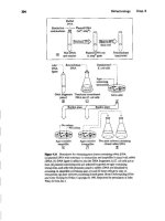
F1guu ZJI Natural tolerances (NT) ~ Ihe darker bands, for a variety of common
mechanical manufacturing processes. Variations

=
the lighter bands (from
MClI1ufacrurmg Processes for Engineering Materials
by Kalpakjian,
©
1997.
Reprinted by permission of Prentice-Hall, Inc., Upper Saddle River, NJ).
bulk shape. Flame cutting could then be followed by a series of machining operations
to obtain further accuracy. These can then be followed by grinding and polishing if
high accuracy and finish are desired by the designer.
In Figure 2.8, the NTs of flame cutting, machining, and grinding are shown,
moving across from left to right with finer accuracy. Several points should be made:
•The designer should realize that these process chains exist, as summarized in
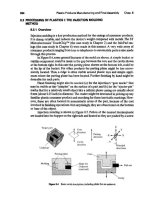
the simple diagram of Figure 2.9.
• Each additional process is needed after a certain transitional tolerance. If the
designer is unaware of these transitions, unnecessary finishing costs may be
created, as shown in Figure 2.10. The other side of this coin is that manufac-
turing costs can he saved if the designer is willing to loosen desired tolerances.
• The manufacturing quality assurance at one step in the process chain must be
carefully executed before moving on to the next process. If a "parent" process
is "ended too early," the next "child" process may have too much or an impos-
sible amount of work to do. (Imagine cleaning a rusty garden tool; heavy
2.3 Question 2: How Much Will the Product Cost to Manufacture
(e)7
37
015
015
Secondary process flat capability
FiJUre2.' Process
chains with

levelsof tojerance
grinding or heavy abrasive papers are needed before moving on to the final
polishing steps.)
2.3.8
Product Life Expectancy
Recall that part strength is listed as the third criterion in Table 2.2. It is related to the
design geometry, tolerances, material selected, and chosen manufacturing method.
These factors also have a coupled influence on the long-term in-service life. Aero-
space and structural engineers are probably the designers who are most concerned
with these long-term properties. Hertzberg (1996) and Dowling (1993) describe the
fatigue properties of metals and polymers. The influences of material composition
and local-geometry effects are also described. A fatigue failure always begins at a
stress concentration. A sharp corner, a small hole, a rapid transition in diameter are
examples of danger zones for crack initiation. Designers in such fields will specify
high integrity grades of steel and aluminum, will choose processes like forging and
forming (rather than casting) to maintain a homogeneous grain structure, and will
specify additional final finishing operations such as grinding and lapping. These
I
Drill
IEDM
I
Broach
Ream
IBm",l
Honing
I
Hole hierarchy
Flat hierarchy
c;ingl
IFinegrind

Broach
IEDMI
I
Mill
!Roughgrjnd
Secondary process hole capability
Surt rougjrin Itr-e tnche
Dtm acc in Hr-s mcnes
Dim ace in 10
_1
inches
Surf rough in Iu-e Inches
38 Manufacturing Analysis: Some Basic Questions for a Start-Up Company Chap. 2
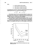
400
Figure2.10 Finishingcostsincreaseasa
part moves from a rough casting.to a
finish-machined part, to fine-honed final
product (from Manufacturing Processes
for Engineering Materials
by
Kalpakjian,
© 1997. Reprinted by permission
of Prentice-Hail, Inc" Upper Saddle
River,NJ).
#"
300
i
~ 200
i
~ 100

additional operations lead to very smooth surfaces that give dramatically improved
long-term fatigue life.
Figure 2.10 illustrates the costs of these additional fine finishing operations.
The additional grind and hone operations add 400% more cost over the as-forged,
or as-cast, surfaces. Even in comparison with turning on a lathe, they add 200 to 300%
more cost. It is not surprising that carefully manufactured aircraft components, or the
surface of a production quality plastic injection mold, are so very expensive.
2.3.9
Lead lime
Lead time is defined for this book as "the number of weeks between the release of
detailed CAD files to the fabrication facility and the actual production of the part."
It is a small subcomponent of the total time-to-market. This broader topic will be
reviewed in greater depth in Section 2.5.For this overview, the important point isthat
lead time is very dependent on the designer's decisions, which then have direct impli-
cations on the choice of manufacturing process. The desired batch size, part geom-
etry, and accuracy are the main factors. As a benchmark, a small batch of medium
complexity metal parts with +/~50 microns (+1- 0.002 inch) accuracy can be
obtained from a production machine shop with a two- to three-week turnaround
time, obviously depending on normal business conditions.
However, several weeks of lead time will be experienced as soon as a serious
mold or die is needed. For the processes like forging, sheet metal forming, and high-
volume plastic injection molding, the die making involves many extra steps. During
die design, factors such as springback for metals and shrinkage for plastics need to
be incorporated. Since the deformation stresses that build up during manufacturing
are high, the die designer also has to create supporting blocks and pressure plates.
The designer will also need to consider parting planes and the draft angles that give
slight tapers to any vertical walls: these are needed to ensure that the part can be
ejected after forming. Unfortunately, perfect analytical models do not exist yet for
2.3 Question 2: How Much Will the Product Cost to Manufacture Ie)?
39

predicting the precise amounts of springback or the best draft angle. This usually
means that handcrafting is needed in the production of the first die. Subsequent trial-
and-error adjustments and iterations to the die surfaces are always needed.
The above paragraph still pertains only to one machine and one process. Several
months of lead time are needed to set up the large-scale FMS systems and high-volume
batches indicated at the bottom right of Figure 2.6.These contain a large number of
manufacturing processes, linked together and scheduled to make complex subassem-
blies.And of course as product complexity and scope increase, the lead time increases
proportionally. At the extreme, for a completely new model of aircraft or automobile,
the lead time from design to first product will run into years rather than months.
2.3.10
Cost Factors Especially Related to Adjoining Parts
The following example shows how design and manufacturing keep changing to suit a
rather complex interaction between (a) the availability of innovative manufacturing
techniques and (b) new economic conditions. In other words, recalling Ayres and
Miller's (1983) quotation in Chapter 1,
"elM
is the confluence of the supply elements and
the demand elements."
TWentyor even ten years ago, it would not have seemed reasonable to machine
very large structures from a solid monolithic slab. However, innovative machining pro-
grams at BoeingAircraft are proceeding in that direction. Inside the ceilingof the plane,
structural members that resemble giant coat hangers are spaced across the plane at
intervals to giveit torsional stability.Today,most are made from many conjoined pieces.
This arrangement is shown in the upper photograph of Figure 2.11. However, newer
designs are favoring machining from one very large solid slab, as shown in the lower
photograph. This eliminates costly and unpredictable joining operations in the factory.
Thomas (1994) has observed that such manufacturing innovations flowing back
into the design phase must be the new way of organizing the relationship between
design and manufacturing. Using Ayres and Miller's definition of CIM we can observe

that the new innovations, or the new supply elements, include:
•Improved cutting tool technology and an understanding of how to control the
accuracy of very high speed machining processes
•The availability of stiffer machine tools and very high speed spindles
•More homogeneous microstructures that give uniformity in large forging slabs
•The ability to carry out comprehensive testing and show that these one-piece
structures are at least if not more reliable than multiple-piece structures.
Meanwhile the new demand elements include:
• Escalating costs of joining and riveting operations, which can only be partially
automated. Specifically these operations often require manual fixturing of the
workpieces
•A preference fOT eliminating multiple fabrication steps, which always demand
more setup, fixturing, documentation, and quality assurance.
• General pressures on the whole airline industry, since deregulation, to cut costs
and yet improve the safety and the integrity of the aircraft.
40 Manufacturing Analysis: Some Basic Questions for a Start-Up Company Chap. 2
FIgure 2.11 Integrated product and process design allows this aerospace
component to be completely machined from the solid as shown in the lower
photograph (counesy of Dr. Donald Sandstrom, The Boeing Company).
These trends introduce a great deal of complexity into the design and manu-
facturing process, but on the other hand, creative companies can exploit them to their
advantage. The conclusion to be drawn is that no single component should be ana-
lyzed and optimized in isolation. There will always be something that can be
improved, simplified, or made cheaper if design and manufacturing are viewed from
a slightly wider system perspective.
2.3.11 Analyzing Costs in Terms of the Profit Potential
Hewlett-Packard's return map (RM) is another method for analyzing design and
manufacturing costs. However, it focuses not just on cost but on these survival
questions:
• How much profit.

aP,
will be made at any given time?
• How long, T
b
,
will it take to make any profit?
Fignre 212 plots the costs or revenues against logarithmic time expelled. The
key curves on the chart (modeled on House and Price, 1991) are:
2.3 Question 2: How Much Will the Product Cost to Manufacture
(en
4'
1,000
Total sales
RF",
return factor at AT after
T
m
'" total investment + AP
atl:1T
after
T
m
total investment
T.
~gure 2.12 Hewlett-Packard's return map (diagram based on House and Price,
1991;Magrab,1997).
• The total investment of dollars starting from the first instant (Te) that engi-
neers start dreaming up the project (see the top of Figure 2.1 at the beginning
of the chapter).
•The total sales that begin as soon as possible after the first product is manu-

factured and sold, T
m'
Note that setting up and debugging the manufacturing
line generate no sales.
•The total profit that starts to be gained at Tb•
The key points on the time axis are:
• Te~the project initiation point. This is followed by product definition, product
development, process planning for manufacturing, setting up machines, debug-
ging the assembly line, and first launch into manufactured product around
point T
m•
•Tm-the
point where real manufacturing begins and products get sold.
• Tb~the
break-even
lime
from the very beginning uf the "conceptual product
definition" to the point where a positive profit occurs
(T
b -
T
e
), Note that the
chart also shows the break-even-after-release time, which measures (T
b
~
T
m)
and focuses more on manufacturing productivity. Obviously, fast production
and high volumes of product are desirable. The goal is to quickly amortize all

the development costs.
• li.T
and li.P-any arbitrary point (AT,AP) beyond the break-even-after-release
time (Tm)where Hewlett-Packard's return factor (RF) is calculated. The RFis
(
Product
definitior
I
Product development
Manufacturing and sales
Total investment
-Break-even time
Total operating
profit
<,
-B'reak-evenafter
I
release
42 Manufacturing Analysis: Some BasicQuestions for a Start-Up Company Chap. 2
calculated by dividing total profits by total investments. The goal is to maxi-
mize
RF
in the shortest time after
T
m'
More importantly, it is also possible to
measure an RF' from the break-even time, T
e•
In terms of profitability for the
whole company,break-even time ismore crucial than break-even-after-release

time. New companies with limited cash flow should focus more on the former
measure.
What is the income stream from the product? The following definitions are
often used:
•Sales price
=
estimated sales price of one unit from company to distributor
(not retail)
•Net sales
=
individual sales price x number of products sold
•Cumulative net sales
=
integrated net sales over several consecutive years
What are the costs of being in business and producing that particular product?
The following definitions are often used:
•Unit cost
=
prime manufacturing and related manufacturing overhead costs of
a single unit of product (see the cost of goods manufactured on the right of
Figure 2.5)
•Cost of the product
=
unit cost x number of products sold
•Development costs
=
conceptual and detailed design
+
launch
+

support
•Marketing costs
=
a percentage of net sales (Magrab, 1997,uses 13%)
•Other promotional and running costs
=
a percentage of net sales (Magrab,
1997,uses 8%)
What is the potential profit or loss? The following definitions are often used:
•Gross margin
=
net sales - cost of product
•Percentage gross margin
=
gross margin
I
net sales x 100%
•Pretax profit
=
gross margin - development costs - marketing costs - other
•Cumulative profit
=
integrated profits (or losses) on a year-by-year basis
Table 2.4 has been reproduced from Magrab (1997) to show some specificfig-
ures. In that example, the first two yean; have no sales. However, the design and
development costs are running up all the time showing a bottom line,
temporary loss
of
$1.6
million.

This particular illustration shows that by the year 2005,the product makes an
impressive profit. But the risks of the first two to three years cannot be emphasized
enough. And what if the customer does not like the product when itis released to the
market? What if the development time is too long and another company launches a
similar product first? Or a better product a few weeks later? The risks of a company
are far too evident here.
Also it is useful to ask, Where will the 1.6 million come from? Obviously from
a loan of some kind (new company) or a strategic investment (larger, existing com-
pany).At what effective interest rate?
8%? 1O%?12%1
What other products might
Year
1997 1998 1999'
2lJlJO
2001 2002 2003 2004 2005
j
= 1
j
= 2
I = 3
J
=4
j
=5
j
=6
j
=7
j
= 8

j
=9
A Sales price
$65.90 $65.90
$67.90 $67.90 $67.90
$67.90 $67.90
B Number of units sold
100,000
250,000
3OO,lJlJO
350,000 250,000
200,000 150,000
C Net sales [=AB] $6,5lXl,000 $16,475,000 $20,370,000
$23,765,000 $16,975,000 $13,580,000 $10,185,000
D Cumulative net sales
[=SUMC(j)] $6,590,000 $23,065,000 $43,435,000
$67,200,000 $84,175,000
$97,755,00 $107,940,000
E Unit cost ttarget} $34.00
$33.50 $33.00 $33.00
$33.50
$34.00 $34.50
F Cost of product sold
[=BEJ
$3,400,000 $8,375,000
$9,900,000
$11,550,000 $8,375,000 $6,800,000 $5,175,000
G Gross margin ($) [=C-F]
$3,190,000 $8,100,000
$10,470,000

$12,215,000
$8,600,000 $6,780,000
~,010,00J
H %grossmargin[=IOOGICJ
48.41%
49.17% 51.40%
51.40%
50.66%
49.93% 49.19%
I Development cost
$8OO,lJlJO
$800,000
$4OO,lJlJO
$50,000
$50,000 $50,000 $50,lXXl $50,000 $50,000
J Marketing(13%nelsales)
[=O.13CJ
$856,700
$2,141,750
$2,648,100 $3,089,450
$2,206,750
$1,765,400 $1,324,050
K Other(8%ofnetsales)
[=0,08CJ $52'1,200 $1,318,000
$1,629,600
$1,901,200
$1,358,000 $1,086,400 $814,800
L Total operating expense
{",I+J+KJ
$800,000

sscicco
$1,783,900
$3,509,750
$4,327,700 $5,040,650 $3,614,750 $2,901,800
$2,188,850
M Pretax profit [=G-LJ
($800,000) ($800,000)
$1,406,100
$4,590,250
$6,142,300 $7,174,350 $4.985,250 $3,878,200
$2,821,150
N %profit[=l00MlCJ
21.34%
27.86% 30,15% 30.19%
29.37%
28.56% 27.70%
o
Cumulative profit
[=SUMMUlJ
($800,000) ($1,600,000)
($193,900)
$4.396,350
$10,538,650
$17,713,000 $22,698,250 $26,576,450 $29.397,600
"Product enters market midyear.
TABLE
2.4 An Example of Magrab's Baseline Hypothetical Profit Model. (Reprinted with permission from Integrated Product and Process Design by
E. 8. Magrab. Copyright CRC Press, Boca Raton, Florida.)
44 Manufacturing Analysis: Some Basic Questions for a Start-Up Company Chap. 2
be launched by <www.start-up-company.com>thatwouldmakelessmoneyoverall

but involve a much lower risk than $1.6 million? What other projects might a large
existing company sponsor? Would another project be more central to the company
mission?
These questions are really beyond the scope of the present book. Economics
by Parkin (1990) or Engineering Economy by Thuesen, Fabrycky, and Thuesen
(1971) have many chapters devoted to such issues as the economic analysis of
alternatives.
2.4 QUESTION 3: HOW MUCH QUALITY 1017
2.4.1 Introduction: Process Quality versus Organizational
Quality
What is quality? How much quality does a product need? Can quality be measured
numerically, andlor does it also involve aesthetic issues? In particular what is the
"cost of quality"? Also, is there a "cost of not enough quality"?
To begin to answer these questions, a definition of quality is needed. In these
next few sections, several definitions will be given.
•The first definition considers a parameter such as the measured diameter of a
manufactured shaft in relation to the desired diameter requested by the
designer. This is one aspect of process quality.
•The second definition considers more global measures of a company's overall
quality. This is more related to organizational quality or total quality manage-
ment (TOM). In Chapter 1,it was emphasized that
u.s.
engineers, particularly
W.E. Deming, were the early advocates of TOM but Japanese companies, such
as Toyota (Ohno, 1988),were the first to passionately apply them. Fortunately,
by 1982,books such as Tom Peters's In Search of Excellence made U.S.manu-
facturers realize what they had to do to restore U.S. manufacturing competi-
tiveness: (a) quality assurance on the factory floor, (b) TQM throughout the
complete organization, and (c) leaner management hierarchies. Garvin (1987)
has described eight aspects of TQM, and they are also evaluated by the Mal-

colm Baldrige Award and the ISO 9000 system. Cole's (1999) recent book
describes the use of such procedures within a "learning organization." These
will be reviewed later in this chapter.
2.4.2 Process Quality on the Factory Floor: Quantitative
Measurements Using Statistical Quality ControlISQC)
Process quality is directly related to the physics of a manufacturing process, specifi-
cally,its inherent accuracy and how well it is controlled.
Imagine a group of friends in a British pub playing darts. Each player is given
three darts. The goal is to hit the bull's-eye with each throw. Each player takes a turn,
and then the round resumes. After an hour of pleasant drinking and playing, how
2.4 Question 3: How Much Quality !OP
45
many bull's-eyes does each player score? And what type of clustering occurs around
the butt's-eyer
• Player One is very experienced and scores many bull's-eyes, In addition, even
when the bull's-eye is not hit, the darts are clustered symmetrically around it
in a small circle 50 millimeters (2 inches) in diameter.
• Player Two is less experienced and scores some bull's-eyes. However, the darts
are scattered all over the board in a much larger circle of diameter 325 mil-
limeters (13 inches). This is about the diameter of the scoring circle of a stan-
dard dart board.
• Player Th:ree has never played before. No bult's-eyes are scored, and to great
laughter, the board is often missed altogether and the darts ricochet onto the
floor.
• Player Four has a strange style. All the darts are grouped together un the left-
hand side of the scoring board (this is the number eleven zone on a standard
dart board). No bull's-eyes are scored. However, the darts are consistently
grouped in a 2-inch diameter circle close to tbc legal edge of the scoring target.
The other players wonder why Player Four just can't pull them all over to the
bull's-eye.

• Player Five is quite good. At the beginning of the evening, many bull's-eyes
create a score ahead of Player Two.But too much beer is consumed, and by the
end of the evening Player Five is much worse than Player Two.
• Player Six is in principle better than Player 'TWo,but this is a player who is
easily distracted by other people in the pub. There are a great number of bull's-
eyes and on average a better clustering than Player Two.However, quite often,
a dart goes way off target. So far off,in fact, that the errors are more dangerous
than those of Player Three.
The obvious point of these entertaining thought experiments is that manufacturing
processes are subject to the same problems.
In the semiconductor industry, many process steps occur: they involve lithog-
raphy machines, dry-etching machines, diffusion chambers, and vapor deposition
machines. All are subject to the inherent behavior seen in the dart players.
In the machine tool industry, imagine now that a circular shaft is being
machined on six different lathes. The shaft might be going into the central axis of a
lawn mower. There is a target dimension of 25 mm or 1inch. The shafts are measured
as they come off the six machines by an automatic touch sensor:
• Machine One is very accurate and repeatable, All the shaft diameters are clus-
tered around the 25 mm or 1 inch target. The spread is 50 microns (0.002 inch).
Machine One is delivering 25 mm shafts with +1-25 microns in their diameter.
• Machine Two is less accurate. The shaft diameters have a much bigger spread,
as much as 500microns (0.02 inch) to give a25 nun diameter (micron
+/-250).
As with the first two dart players, Machine Two is less accurate than Machine
One. Perhaps Machine Two can be used for some rough cutting on cylindrical
46
Manufacturing Analysis: Some BasicQuestions for a Start-Up Company Chap. 2
parts where accuracy is not critical. Or, more importantly, the SQC Quality
Assurance Department can recommend machine maintenance to improve the
machine.

•Machine Three has hopeless accuracy.Some parts are so far off the 25 mm or
1 inch target that the Quality Assurance Department stops any kind of pro-
duction on the machine and begins serious maintenance work. Perhaps an
actuator or lead screw is damaged, and occasionally, the machine sticks in
place-way off from its desired settings.
•Here is an important question: What is the difference between accuracy and
precision? Machine Four, like Player Four, demonstrates this difference when
compared with Machine One, or Player One. The results of Machine Four
demonstrate great precision. However, the precision is demonstrated in the
wrong place. Something is wrong with the machine's ability to locate an accu-
rate location. Perhaps a fixture slips right at the beginning of a batch run. The
first shaft is incorrect right from the beginning, but all shaft diameters cluster
around that incorrect location.
• Machine Five starts off well,but tools wear out (on a lathe) or the alignment
drifts (on a lithography machine) and the process deteriorates. The SQC team
must recognize the deteriorating factor and fix it.
•Machine Six is quite good overall, but occasionally a really poor part is pro-
duced. Perhaps this is a machine with a controller error, which shows a short
circuit and causes major errors from time to time.
For this example, the data on the dimensions of the shafts would be monitored and
overseen by a Quality Assurance Department. The results would be statistically ana-
lyzed and stored in extensive computer databases.
These statistical quality control (SOC) databases are the key to maintaining
the highest levels of quality assurance. They provide the information for careful
machine adjustments, machine-maintenance scheduling, timely reporting of errors
or drifting behavior, and machine diagnostics. Recommendations on scheduled
maintenance for a particular machine can also be tied into the factory scheduling.
Such quality assurance can also include the
Pokayoke
approach (Ohno,

1988;
Black, 1991).
Pokayoke
in Japanese simply means "defect free." It can be applied to
machinery design where some additional devices are added to a machine to prevent
an operator from making a mistake like loading a bar in the wrong way around.
Finally,the quality assurance methods might include the formal techniques of
Taguchi. Taguchi
methods focus on the types of noise in a manufactured product and
then proceed to reduce their occurrence by documented statistical means. In addi-
tion,
Taguchi
methods document the lost time that the consumer of the product con-
sur-res,getting the product up and running and/or getting it repaired at some later
date. All such problems are then traced back through the factory to the source of the
noise and allocated a cost function.
This is not "rocket science." Much of it is commonsense quality assurance. In
fact, it isno different from carefully maintaining an automobile; checking the oil,fol-
2.4 Question 3: How Much Quality 10)1
41
lowing the recommended maintenance schedule, fixing problems before they lead to
a major breakdown, scheduling the maintenance when life is not too hectic.
2.4.3
"Specification Limits" versus "Process Control (PC)
Limits"
It is important to understand two definitions that are at first glance similar but that
are "on different sides of the CAD/CAM fence":
• The specification limits set by the designer (often called "the specs" for short)
•The process control limits t'iat are inherent to the manufacturing process being used
Within the "specs" there is an important definition:

• Tolerance: which is related to the designer's needs. The tolerance might be
equal on each side of the "target dimension." This is called a "bilateral toler-
ance spec." Note that there are many cases where the tolerance will deliber-
ately not be symmetrical about the mean. Often shafts will need to fit and
rotate in a central bearing. Thus the shaft cannot be too big without jamming.
But it could be a little smaller without a problem. In the example above per-
haps the tolerance would he written 25 mm
(+0/-50
microns).
Within the process control Inuits there are other important definitions:
• The mean value: such as the mean value of all the cylindrical shafts made. For
reference, the value of (x) at the mean value is assigned
~X'
In Figure 2.13, 13
mm is the mean value.
• The variance around this mean value. This is the same as the natural tolerance
(NT) for the process (not the designer's tolerance). In standard SQC moni-
toring, a value of {NT= 6a
=
+1-
So] is commonly used. It represents each
side of the Gaussian or bell-shaped normal distribution curve shown in Figure
2.13. The ranges of diameter starting from the left tail might be [12.950 to
12.955J, [12.955
:0
12.960], and so forth. Next, the histogram plots the number
of shafts in each band all across to the right side tail.
If the company accepts all the shafts of diameter within
(6u
=

+1-
So}, then
the rejection rate will be 27 out of 10,000 parts. If the company accepted
(120"
=
+
1-
Sc}, then the rejection rate would be 2 out of 1 billion parts.
The desired accuracy-the specs-is summarized in the lower part ofFigure 2.13:
it is the range given by the upper specification limit minus the lower specification limit,
namely (USL - LSL). This might simply be the range of acceptable diameters of the
metal shaft to be used for the central axle of a lawn mower. The ideal diameter and
allowable (USL~ LSL) willbe set by the designer based on functional considerations.
Next, it is common sense to choose a manufacturing process that has the right
capability. Put in other words, its accuracy and NT should match the designer's
demands. Ideally, the designer's value of
(USL-LSL)
should be wider than the
achievable +1-3rr (or NT
=
Sc} of the manufacturing process.
10
48 Manufacturing Analysis: Some Basic Questions for a Start-Up Company Chap. 2
12.95
13.00
Diameter of shafts (mm)
(a)
-4<7-3 -2
-1
0

+1
+2 +3 +4<1
(b)
(USL- LSL)l
(USL-LSL)z
(c)
13.05
F'ipre1.13 lheupperdiagram(a)is
from the manufacturina
prouss
itself
showing data clustered around a mean
shaft diameter of 13 mm. In standard
statistical quality control (SOC) work the
Gaussian or bell-shaped normal curve is
assumed, as shown in (b), meaning that
99.73% of the manufactured parts will lie
inside the range 6c:r""
+1-
3a. The lower
diagram (.:) represents the designer's
desired range. The upper specification
limits (USL) and lower specification
limits (LSL) are shown. In one case,
(USL-
LSL)l is the same as the
manufacturing tolerance: this represcnts
C
p
=

1 and is the minimum acceptable
condition but not really desirable
because, with manufacturing capability of
+/-
317,some parts are certain to faU
outside the designer's specification. In
the second case.
(USL-
LSLh is twice as
large meaning that
C
p
"'-
2.This is more
desirable. Note, however, if C
p
gets too
large, then the chosen manufacturing
process may be "too good" for the rather
loose constraints set
by
the designer.
(diagrams adapted from Kalpakjian,
1997,and DeVoret al., 1992)
Diameterofshafts(mm)
2.4 Question 3: How Much Quality (Q)7
49
Speaking colloquially, to build a precision telescope with tight tolerances and
small values of (USL~LSL), nobody would go into their basement and use an old
hacksaw and blunt drills that have a large value of NT. Surprisingly though, many

manufacturers do struggle with the wrong manufacturing process or wom-out tools
to try and satisfy a designer's needs. Likewise, some designers specify values of
(USL- LSL) that might be "too good" for the needs of the part being designed: in
this scenario, to achieve the tolerances, the manufacturer may have to follow stan-
dard milling or turning operations with a costly finishing process such as precision
grinding or even polishing.
2.4.3.1 Process Capability Index, C
p
The process capability divides the range between the upper arid lower specification
limits (l)SL~ LSL) by the width of the bell-shaped curve. Standard SQC uses +
1- 30'
(namely,
i
t-
3 standard deviations). This measure is known as
C
p
:
USL - LSL
C ~
p
6<r
x
(2.2)
The minimum acceptable value for C
p
is considered to be 1, but as can be seen in
Figure 2.13 a value between 1 and 2 is more desirable.
2.4.3.2 Process Capability Index, C
pk

The preceding discussions basically assume that the mean value of the manufac-
turing process coincides with the desired size of the part set by the designer. In other
words, it assumes that a
+/-
Sc "viewing window" on the manufacturing process
coincides with a (USL- LSL) "viewing window" from the designer.
However, what if this is not the case? Recall Dart Player Four: the darts are all
tightly spaced in a small "viewing window," but the center of the window has drifted
way off target. Machine Four's shafts on the extreme left of the tail will soon be in
error. Following the example given by Devor, Chang, and Sutherland (1992), sup-
pose the ideal size of a shaft, as set by a designer, is 145millimeters.Additionally.sup-
pose that although a chosen lathe operation is more than capable of giving the
desired SQC constraint of +/- So. the tool post on the lathe has been distorted and
all the components have shifted in size, meaning that the mean value is 130 millime-
ters not 145 millimeters. To account for such "drift" of the mean value it is now
common for manufacturers to use a capability index referred to as
C
pk
•
The value of
C
pk
relates the actual process mean to the nominal value of the specification.
For specifications in which the designer sets a desired value and then sets the
same
+/-
tolerance on each side (recall this is called a bilateral spec),
C
pk
is defined

in the following manner. First, it is necessary to determine the relationship between
the process mean
IJ.x
and the specification limits in units of standard deviations:
(2.3)
The minimum of these two values is selected. The reader might pause
fOT
a
moment and think about why this is the case. The answer is as follows: if the shaded
50
Manufacturing Analysis: Some Basic Questions for a Start-Up Company Chap. 2
curve in Figure 2.14 "drifts" to either end of the set range, it is desirable to look at
the "worst case." The schematic figure shows the manufacturing process drifting to
the left-hand side, and so manufactured parts in the left side of the tail will "go out
of spec" first. The analysis must therefore consider how close the Gaussian curve is
to the left side, LSL
=
100 mm.
Zmin
=
minlZuSL, or( -
zLSdl.
(2.4)
The
C
pk
index is then found by dividing this minimum value by 3.The division
is by 3 because this represents one side of the bell-shaped curve or the distance
between the mean value,
~x,

and either LSL or USL depending on which way the
"drift" occurs:
(2.5)
In manufacturing,
C
pk
should be ~1.00 for the process capability to be accept-
able. Again following the example of
Devor,
Chang, and Sutherland (1992), consider
that the process mean has drifted and is located at 130,somewhat away from the nom-
inal of 145,with a standard deviation of
IJ"x
=
10.The calculations proceed as follows:
ZUSL ~ 190 ~ 130
~6
ZLSL ~ 100 ~ 130
~3
Zmm ~
min[16,
0'(-
(-3111J
~3
c.;
= ~
~ 1.00
LSL
USL
Figure 2.14

The manufacturing process
may "drift" due to macroscopic errors,
say in setup, fixturing, temperature
control, and the like. In the example
above, the process is drifting toward the
designer's LSL
=
100. It could mean that
although the process is giving good
performance from a viewpoint of
+/-
So, some of the samples in the left-side
"tail't will soon he out of spec. The
C
pk
evaluation considers this drift (courtesy
of DeVor, Chang, and Sutherland, 1992).
130 145
190
2.4 Question 3: How Much Quality (Q)?
51
However, if the process mean were recentered at the nominal of 145,then:
190 - 145
ZUSL= I0-
~ 4.5
100 - 145
ZLSL= 10-
~ - 4.5
2
m

," ~
min[!4.5, 0'1-(- 4.5))
11
~ 4.5
4.5
C
pk
=)
~ 1.50
The example shows that by recentering the process, the value of C
pk
would be
increased by 50%.
2.4.4 Motorola's 6 Sigma Program
Six sigma quality is a phrase made famous by Motorola once it decided to refocus on
quality in the late 1970s and early 1980s.It is a quality assurance program that has
the goal of reducing the defective parts in a batch to as low as 3.4 parts per million.
Of more academic interest is the precise way in which Motorola implements
this quality standard, which is under some scrutiny from several statisticians
(Tadikamalia, 1994). A rigorous interpretation of 6 sigma really translates to 2
defects per billion parts made. The brief explanation is as fulluws, and it all boils
down to whether the process is allowed to stay centered or not on the desired mean
value (Figure 2.15).
First, consider the production of a million components using a manufacturing
process that is centered on the mean [i.e the target) value. The area under the
normal curve can be calculated for various sigma bands. If we consider the two ver-
tical lines that can be drawn at
+/-
4.5 sigma each side of center, then 6.8 compo-
nents per million will lie in the tails of such a curve, with 3.4 on each side. Clearly, this

is a much tighter tolerance than was allowed in the +1- 3 sigma bands shown in
Figure 2.13.
What happens if the process drifts off-center? Let us say that the center of the
normal curve drifts by 1.5 sigma, this time to the right. If this second curve is still
viewed through a window that is centered on the original origin and is still +1- 4.5
sigma wide, there will be virtually no defects in the left-side tail but a rather large
number in the right-side tail: 1,350 to be exact.
However, if this shifted curve is viewed through a much wider window (a
window that is
+1-
6 sigma wide, centered on the original origin), the analysis
returns to a more favorable view with only very few data in the tails. In this case these
tails will contain 3.4 parts per million, probably all in the right-side tail. Actually,
52
Manufacturing Analysis: Some Basic Questions for a Start-Up Company Chap. 2
I
Aim: 3.4 parts per million. quoted as
00.1
Conclusion'
When centered, the 4.50"lines give 3.4 parts/million on each side
When offset 1.50-,the 6.00-lines give 3.4 parts/million total.
Figure2.15 Motorola's 6-sigma quality assurance method.
there is an infinite combination of "m-sigma offset plus n-sigma viewing window"
ways of staying at a quality performance of 3.4 defects per million.
The positive outcome of all this is that Motorola is rightly known for excellent
products with less than 3.4 defective parts per million. It is this quantitative number
that should be focused on as the benchmark rather than the rigorous definition of 6
sigma. However, the statisticians do have a point when they wonder why Motorola
seems to allow a monitoring scheme in which some of its manufacturing processes
might be allowed to drift off-center.

2.4.5 Summary on Process Quality
The best industry practice from a statistical point of view is to keep careful track of
both the process mean and the process variance.
The process variance can be improved by (a) creating quality circles (groups of
engineers who work diligently on a machine performance to improve process
physics) and (b) investing in new capital equipment that ismore precisely controlled.
Both these solutions are quite expensive and time-consuming. Again it relates to the
dart players: Player Two has to gain more experience, put in more training time, and
I part 3.4 parts
per~illionpe[/million_
Process
on target
3.4 pa~ts 1 part
-'per milli.onper billion
1,350parts:
.oer mtnton
I
3.4 parts
per million
1.5" Offset
2.4 Question 3: How Much Quality
(Q)1
53
try to be as good as Player One. Machine Two has to be studied and modified in cer-
tain aspects. Or it has to be sold and replaced with a better one that can deliver the
desired accuracy.
The process mean, however, can often be addressed more cheaply by moni-
toring the output continuously and using the statistics to keep the mean of each batch
centered on the target value. Measured errors in the process mean or target value
can often be traced to a fixed offset. This might be related to a misoriented fixture or

lithography mask in semiconductor manufacturing, or to a worn cutting tool that has
not been adjusted from one batch run to the next.
As one might expect,
both
the mean and the variance can be thrown off in some
cases. Perhaps a wide variance in the hardness of an incoming work material from an
unreliable subvendor will cause scattered results plus tool wear, which will quickly
move the mean value as well.Thus in conclusion there is no quick fix to obtaining 3.4
defects per million parts. But companies that want to stay in front obviously have to
be part of this goal, refining their techniques in away that really improves their prod-
ucts at an appropriate level of cost.
2.4.6 The "Bigger Picture"-organizational Quality
The Motorola view is that quality assurance touches all aspects of product realiza-
tion, not just the factory floor itself. When analyzed "in the large" manufacturing
becomes a complex art form. Full-scale industrial design of both the product itself
and the production processes that will fabricate the product relies on a huge team of
people ranging from classical mechanical and electrical engineers, to marketing
experts, to venture capitalists, to industrial psychologists, to advertising executives.
Not only does manufacturing in the large encompass the complete assembly line for
a Sony Walkman, or the much larger assembly line for a Ford Mustang, or the
gigantic assembly hangers for a Boeing 777,but it also encompasses market analysis
and consumers' reaction.
Manufacturing in the large can be effective only in the context of rigorous
quality assurance within a "learning organization." Cole (1999) distinguishes orga-
nizational/earning from individual/earning by contrasting two social styles. Indi-
vidual learning can be applied to one person or to one factory unit, but the key thing
is that there are walls around the unit, almost related to a kind of protectionism
tinged with paranoia. The old-style British Trade Union attitude seems to capture
this the most: craftspeople jealously guarding their secret techniques, and factory
units operating for their own bottom line and not worrying about what comes next.

One industrial case study included a metal-extrusion unit that manufactured bar
stock that was geometrically correct but so nonuniformly tempered that the down-
stream machine shop could not meet production schedules. In the old days the har-
ried machine shop had to take care of this problem alone, while the extrusion unit
celebrated record production.
With organizational learning, a problem such as the one above becomes
everyone's problem, including the sales force. This cooperative attitude toward
quality was a very important change in the way U.S. companies began to operate
during the period after 1980. It became known as total quality management (TOM).