Aluminium Design and Construction - Chapter 10 pps

CHAPTER 10

Calculation of section
properties
10.1 SUMMARY OF SECTION PROPERTIES USED
The formulae in Chapters 8 and 9 involve the use of certain geometric
properties of the cross-section. In steel design these are easy to find, since
the sections used are normally in the form of standard rollings with
quoted properties. In aluminium, the position is different because of the
use of non-standard extruded profiles, often of complex shape. A further
problem is the need to know torsional properties, when considering lateral-
torsional (LT) and torsional buckling. The following quantities arise:
(a) Flexural S Plastic section modulus;
I Second moment of area (inertia);
Z Elastic section modulus;
r Radius of gyration.
(b) Torsional St Venant torsion factor;
I
P
Polar second moment of area (polar inertia);
H Warping factor;
X
Special LT buckling factor.
The phrase ‘second moment of area’ gives a precise definition of I and I
p
.
However, for the sake of brevity we refer to these as ‘inertia’ and ‘polar
inertia’.
10.2 PLASTIC SECTION MODULUS
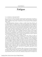
10.2.1 Symmetrical bending
The plastic modulus S relates to moment resistance based on a plastic

pattern of stress, with assumed rectangular stress blocks. It is relevant
to fully compact sections (equation (8.1)).
Firstly we consider sections on which the moment M acts about an axis
of symmetry ss (Figure 10.1(a)), which will in this case also be the neutral
Copyright 1999 by Taylor & Francis Group. All Rights Reserved.
axis. The half of the section above ss is divided into convenient elements,
and S then calculated from the expression:

(10.1)

where A
E
=area of element, and y
E
=distance of element’s centroid E above
ss. The summation is made for the elements lying above ss only, i.e. just
for the compression material (C).
Figure 10.1(b) shows another case of symmetrical bending, in which
M acts about an axis perpendicular to the axis of symmetry. The neutral
axis (xx) will now be the equal-area axis, not necessarily going through
the centroid, and is determined by the requirement that the areas above
and below xx must be the same. S is then found by selecting a convenient
axis XX parallel to xx, and making the following summation for all the
elements comprising the section:

(10.2)

where A
E
=area of element, taken plus for compression material (above

xx) and negative for tensile material (below xx), and Y
E
=distance of element’s
centroid E from XX, taken positive above XX and negative below.
The correct answer is obtained whatever position is selected for XX,
provided the sign convention is obeyed. It is usually convenient to
place XX at the bottom edge of the section as shown, making Y
E
plus
for all elements. No element is allowed to straddle the neutral axis xx;
thus, in the figure, the bottom flange is split into two separate elements,
one above and one below xx.
10.2.2 Unsymmetrical bending
We now consider the determination of the plastic modulus when the
moment M acts neither about an axis of symmetry, nor in the plane of such
an axis. In such cases, the neutral axis, dividing the compressive material
Figure 10.1 Symmetric plastic bending.
Copyright 1999 by Taylor & Francis Group. All Rights Reserved.
(C) from the tensile material (T), will not be parallel to the axis mm
about which M acts. The object is to determine S
m
, the plastic modulus
corresponding to a given inclination of mm.
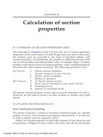
Consider first a bisymmetric section having axes of symmetry Ox
and Oy, with mm inclined at to Ox (Figure 10.2(a)). The inclination of
the neutral axis nn can be specified in terms of a single dimension w as
shown. Before we can obtain the plastic modulus S
m
for bending about
mm, we must first find the corresponding orientation of nn (i.e. determine

w). To do this, we split up the area on the compression side into convenient
elements, and obtain expressions in terms of w for the plastic moduli
S
x
and S
y
about Ox and Oy, as follows:

(10.3)

where A
E
=area of an element, and x
E
, y
E
=coordinates of the element’s
centroid E referred to the axes Ox and Oy.
In each equation, the actual summation is just performed for the
compression material (i.e. for elements lying on one side only of nn).
The correct inclination of nn, corresponding to the known direction of
mm, is then found from the following requirement (which provides an
equation for w):
S
y
=S
x
tan . (10.4)

Having thus evaluated w, the required modulus S

m
is obtained from
(10.5)

The procedure is similar for a skew-symmetric section (Figure 10.2(b)),
where a single parameter w is again sufficient to define the neutral axis
nn. In this case, the axes Ox, Oy are selected having any convenient
orientation. The above equations (10.3)–(10.5) hold good for this case,
and may again be used to locate nn and evaluate S
m
.
Figure 10.2 Asymmetric plastic bending.
Copyright 1999 by Taylor & Francis Group. All Rights Reserved.
We now turn to monosymmetric sections (Figure 10.2(c)). The above
treatment holds valid for these in principle, but the calculation is longer,
because we need two parameters (w, z) to specify the neutral axis nn. The
whole section is split up into convenient elements, none of which must
straddle nn. A convenient pair of axes OX and OY is selected, enabling
expressions for S
x
and S
y
(in terms of w and z) to be obtained as follows:

(10.6)

where: A
E
=area of an element taken positive for compression material
and negative for tensile, and X

E
, Y
E
=coordinates of an elements’s centroid
E referred to the axes OX and OY, with signs taken accordingly. The
summations are performed for the whole section. The dimensions w
and z (defining the position of nn) are then obtained by solving a pair
of simultaneous equations based on the following requirements:
1. The areas either side of nn must be equal.
2. Equation (10.4) must be satisfied.
Having thus found w and z, the required modulus S
m
is determined from
expression (10.5) as before. The right answer will be obtained, however
the axes OX and OY are chosen, provided all signs are taken correctly.
Unsymmetrical sections can be dealt with using the same kind of
approach.
10.2.3 Bending with axial force
The reduced moment capacity of a fully compact section in the presence
of a coincident axial force P can be obtained by using a modified value
for the plastic section modulus, as required in Section 9.7.5 (expressions
(9.22)) and also in Section 9.7.7(1).
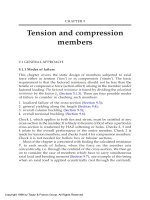
Consider first the symmetrical bending case when the moment M
acts about an axis of symmetry ss (Figure 10.3(a)). The aim is to find
the modified plastic modulus S
p
which allows for the presence of P.
The figure shows the (idealized) plastic pattern of stress at failure
with assumed rectangular stress-blocks, in which we identify regions
1, 2, 3. Region 2 extends equally either side of ss, the regions 1 and

3 being therefore of equal area. Region 2 may be regarded as carrying
P, while 1 and 3 look after M. Referring to Section 9.7.5 the stress on
region 1 is assumed to be p
a
for check A (localized failure), or p
o
for
check B (general yielding). The height of the neutral axis nn is selected
so that the force produced by the stress on region 1 (=its area×p
a
or
p
o
) is equal to
m
P. The required value of S
p
is then simply taken as the
plastic modulus contributed by regions 1 and 3. Note that the value
thus obtained is slightly different for the two checks. (P is axial force
under factored loading.)
Copyright 1999 by Taylor & Francis Group. All Rights Reserved.
A similar approach is used for the other symmetrical case, namely
when M acts about an axis perpendicular to ss (Figure 10.3(b)). In defining
region 2, it is merely necessary that, apart from having the right area (to
carry
m
P), it should be so located that regions 1 and 3 are of equal area.
Figure 10.3(c) shows an example of unsymmetrical bending, where
the moment M acts about an axis mm inclined at to the major principal

axis of a bisymmetric section, again in combination with P. In this case,
the modified plastic modulus, which we denote by S
pm
, is a function of
P and . Two parameters (w, z) are now needed to define the neutral axis
nn, as shown, and these may be found from the requirements that: (1)
region 2 must have the right area, and (2) the values of S
x
and S
y
provided
by regions 1 and 3 (hatched areas) must satisfy equation (10.4). Having
thus located nn, and the extent of the three regions, the required value
of S
pm
is found by using an expression equivalent to equation (10.5).
An identical approach can be used for a skew-symmetric profile,
where again two parameters are sufficient to define nn. The same principles
apply to other shapes (monosymmetric, asymmetric), but the working
becomes more laborious.
10.2.4 Plastic modulus of the effective section
The plastic modulus should when necessary be based on an effective
section, rather than the gross one, to allow for HAZ softening at welds
and for holes (Section 8.2.4). In considering the HAZ effects, alternative
methods 1 and 2 are available (Section 6.6.1).
In method 1, we take a reduced or effective plate thickness k
z2
t in
each nominal HAZ region, instead of the actual thickness, and calculate
S accordingly.

Method 2 is convenient for a section just containing longitudinal welds.
For bending about an axis of symmetry, it consists of first obtaining S for
the gross section, and then deducting an amount yA
z
(1-k
z2
) at each HAZ due
to the ‘lost area’ there, where A
z
is the nominal softened area and y the
Figure 10.3 Plastic bending with axial load. NA=neutral axis. Hatched areas carry the
moment.
Copyright 1999 by Taylor & Francis Group. All Rights Reserved.
distance of its centroid from the neutral axis. For a relatively small longitudinal
weld, there is no need to have a very precise value for y. The above approach
may also be used when bending is not about an axis of symmetry, except
that the lost areas now affect the location of the neutral axis.
10.3 ELASTIC FLEXURAL PROPERTIES
10.3.1 Inertia of a section having an axis of symmetry
The inertia I (second moment of area) must generally be determined
about an axis through the centroid G of the section.
To find I
xx
about an axis of symmetry Gx we split up the area on one
side of Gx into convenient elements (Figure 10.4(a)), and use the
expression:

(10.7)

where: I

Exx
=an element’s ‘own’ inertia about an axis Ex through its centroid
E parallel to Gx, A
E
=area of the element, and y
E
=distance of E from the
main axis Gx. The summations are made for the compression material
(C) only.
Figure 10.6 shows various common element shapes, for which the
value of I
Exx
and the position of E may be obtained by using the expressions
in Table 10.1.
When bending does not occur about an axis of symmetry, but about
one perpendicular thereto (Figure 10.4(b)), we have first to locate the
neutral axis, i.e. find the position of the centroid G. To do this, we select
any convenient preliminary axis XX parallel to the axis of bending. The
distance Y
G
that the neutral axis lies above OX is given by:

(10.8)
Figure 10.4 Elastic symmetric bending.
Copyright 1999 by Taylor & Francis Group. All Rights Reserved.
where A
E
=area of the element (normally taken positive), and Y
E
=distance

of the element’s centroid E from XX taken positive above XX and
negative below.
The summations are performed for all the elements. The correct position
for the neutral axis is obtained, however XX is chosen, provided the
sign of Y
E
is taken correctly. A negative value of Y
G
would indicate that
the neutral axis lies below XX. There are then two possible formulae
for I
xx
which both give the same answer:
Either
(10.9)
or
(10.10)

Expression (10.9) is the one taught to students. Expression (10.10) is
more convenient for complex sections because a small design change to
one element does not invalidate the quantities for all the others.
10.3.2 Inertias for a section with no axis of symmetry
When the section is skew-symmetric or asymmetric (Figure 10.5) we usually
need to know the inertias about the principal axes (Gu, Gv), known as
the principal inertias (I
uu
, I
vv
). The procedure for finding the orientation
of the principal axes and the corresponding inertias is as follows:

1. Select convenient preliminary axes Gx and Gy through the centroid
G, with Gy directed 90° anti-clockwise from Gx.
2. Calculate the inertia l
xx
. using equation (10.9) or (10.10). Use an
equivalent expression to calculate I
yy
.
3. Calculate the product of inertia I
xy
(Section 10.3.3).
4. The angle a between the major principal axis Gu and the known axis
Gx is then given by:
(10.11)
Figure 10.5 Elastic bending, principal axes.
Copyright 1999 by Taylor & Francis Group. All Rights Reserved.
If is positive we turn clockwise from Gx to find Gu; if negative
we turn anticlockwise. The minor principal axis G is drawn
perpendicular to Gu.
5. Finally, the major and minor principal inertias are calculated from:
(10.12)
where


Figure 10.6 Elements of sections.
Copyright 1999 by Taylor & Francis Group. All Rights Reserved.
Table 10.1 Elements of sections—properties referred to axes through element centroid
Notes. 1. Refer to Figure 10.6 for element details.
2. In case 2 and 11–14 it is assumed that t is small relative to b or r.
Copyright 1999 by Taylor & Francis Group. All Rights Reserved.

10.3.3 Product of inertia
The product of inertia I
xy
, appearing in Section 10.3.2, can be either
positive or negative. It may be calculated using the following expression
in which the summations are for all the elements of the section:

(10.13)

where I
Exy
=an element’s ‘own’ product of inertia, referred to parallel
axes Ex and Ey through its centroid E, A
E
=area of the element (taken
positive), and X
E
, y
E=
coordinates of E referred to the main axes Gx and
Gy, with strict attention to signs.
Table 10.1 includes expressions for I
Exy
for the common element shapes
shown in Figure 10.6. In applying these, it is important to realize that
I
Exy
can be either positive or negative, depending on which way round
the element is drawn. As drawn in the Figure, it is positive in every
case. But if the element is reversed (left to right) or inverted, it becomes

negative. If it is reversed and inverted, it becomes positive again.
10.3.4 Inertia of the effective section
The elastic section properties should when necessary be based on an
effective section, to allow for HAZ softening, local buckling or holes.
There are two possible methods for so doing.
In method 1, we take effective thicknesses in the nominal HAZ regions
(Section 6.6.1) and effective stress blocks in slender elements (Chapter
7), I being calculated accordingly. The HAZ softening factor k
z
is put
equal to k
z2.
If the section is semi-compact, there are no slender elements
and thus no deductions to be made for local buckling.
In method 2, we treat the effective section as being composed of all
the actual elements that constitute the gross section, on which are then
super-imposed appropriate negative elements (i.e. ‘lost areas’). In any
HAZ region, the lost area is A
z
(1-k
z2
). In a slender element it consists of
the ineffective material between effective stress blocks (internal elements),
or at the toe (outstands). I is obtained basically as in Section 10.3.1 or
10.3.2, combining the effect of all the positive elements (the gross section)
with that of the negative ones (the lost areas), and taking A
E
, I
Exx
, I

Eyy
and I
Exy
with reversed sign in the case of the latter. In considering the
lost area due to softening at a longitudinal weld, there is no need to
locate the HAZ’s centroid with great precision.
Method 2 tends to be quicker for sections with small longitudinal
welds, since it only involves a knowledge of A
z
without having to find
the actual distribution of HAZ material.
Copyright 1999 by Taylor & Francis Group. All Rights Reserved.
10.3.5 Elastic section modulus
The elastic modulus Z, which relates to moment resistance based on an
elastic stress pattern, must always be referred to a principal axis of the
section. It is taken as the lesser of the two values I/y
c
and I/y
t
, where I
is the inertia about the axis considered, and y
c
and y
t
are the perpendicular
distances from the extreme compressive and tensile fibres of the section
to the same axis. HAZ effects, the presence of holes and local buckling
should be allowed for, when necessary, by basing I and hence Z on the
effective section.
10.3.6 Radius of gyration

This quantity r is required in calculations for overall buckling. It is
simply taken equal to (I/A) where I is the inertia about the axis considered
and A the section area. It is generally based on the gross section, but
refer to Section 9.5.4 for sections containing very slender outstands.
10.4 TORSIONAL SECTION PROPERTIES
10.4.1 The torque-twist relation
The torsional section properties , I
p
, H and
x
are sometimes needed
when checking overall member buckling. They should be based on the
gross cross-section.
In order to understand the role of and H, it is helpful to consider
the simple form of the torque-twist relation for a structural member,
when subjected to an axial torque T:

(10.14)

where =rotation at any cross-section, =rate of change of with respect
to distance along the member (‘rate of twist’), G=shear modulus of the
material, and =St Venant torsion factor.
This equation would be valid if there were no restraint against warping,
the idealized condition whereby the torque is applied in a way that
leaves the end cross-sections free to distort longitudinally, as illustrated
for a twisted I-section member in Figure 10.7(a).
Figure 10.7 Torsion of an I-beam: (a) ends free to warp; (b) warping prevented.
Copyright 1999 by Taylor & Francis Group. All Rights Reserved.
Usually the conditions are such as to provide some degree of restraint
against warping, leading to an increase in the torque needed to produce

the same total twist. Figure 10.7(b) shows an extreme case in which the
warping at the ends is completely prevented. In any case where warping
is restrained, referred to as ‘non-uniform torsion’, the torque-twist relation
becomes:
(10.15)

where
= third derivative of , E=elastic modulus of the material, and
H=warping factor.
The quantity is always of opposite sign to , so that the EH-term
in fact represents an increase in T as it should. The section property
roughly varies with thickness cubed, whereas H is proportional to
thickness. The contribution of the EH-term therefore becomes increasingly
important for thin sections.
Equation (10.15) also applies when the torque varies along the length,
which is what happens in a beam or strut that is in the process of
buckling by torsion. However, ‘type-R’ sections composed of radiating
outstands (Figure 9.7) are unable to warp. For these, H is therefore zero
and equation (10.14) is always valid.
10.4.2 Torsion constant, basic calculation
The torsion constant for a typical non-hollow section composed of
flat plate elements (Figure 10.8(a)) can be estimated by making the
following summation for all of these:

(10.16)

where b and t are the width and thickness of an element . For a curved
element, it is merely necessary to measure b around the curve. If the
Figure 10.8 Sub-division of the section for finding .
Copyright 1999 by Taylor & Francis Group. All Rights Reserved.

thickness t of the element varies with distance s across its width, the
contribution dI is taken as:

(10.17)

Hollow sections have a vastly increased torsional stiffness, as compared
with non-hollow ones of the same overall dimensions. Even so, it is
occasionally possible for them to fail torsionally, as when a deep narrow
box is used as a laterally unsupported beam. To find for a hollow
section (Figure 10.9), we simply consider the basic ‘torsion box’ (shown
shaded) and ignore any protruding outstands. is then given by:

(10.18)
where A
b
=area enclosed by the torsion box measured to mid-thickness
of the metal, s=distance measured around the periphery of the torsion
box, and t=metal thickness at any given position s.
The integral in the bottom line of equation (10.18) is evaluated all
around the periphery of the torsion box. For a typical section, in which
the torsion box is formed of flat plate elements, it can be simply obtained
by summing b/t for all of these.
10.4.3 Torsion constant for sections containing ‘lumps’
The torsional stiffness of non-hollow profiles can be much improved
by local thickening, in the form of liberal fillet material at the junctions
between plates, or bulbs at the toes of outstands. To find for a
section thus reinforced we again split it up into elements and sum the
contributions (Figure 10.8(b)). For a plate element, is bt
3
/3 as

before; while for a ‘lumpy’ element, it may be estimated from data
given below or else found more accurately using a finite-element
program.
Figure 10.9 Basic torsion box for hollow section,
Copyright 1999 by Taylor & Francis Group. All Rights Reserved.
Figure 10.10 Torsion. Section reinforcement covered by expression (10.19) and Table 10.2.
Table 10.2 Torsion constant. Factors used in finding dI for certain types of section
reinforcement
Notes. 1. The table relates to expression (10.19).
2. Refer to Figure 10.10 for geometry and definition of N.
Copyright 1999 by Taylor & Francis Group. All Rights Reserved.
Figure 10.10 shows a selection of junction details and also two quasi-
bulbs. For any of these the contribution may be found using a
general expression:
=[(p+qN+r)t]
4
(10.19)

where N=geometric factor (see Figure 10.10), t=adjacent plate thickness,
and p,q,r=quantities given in Table 10.2, valid over the ranges indicated.
Note that for each detail equation (10.19) covers the area shown
hatched in Figure 10.10, with the adjacent plate element or elements
terminated a distance t or T from the start of the actual reinforcement.
This treatment is based on results due to Palmer [28] before the days
of computers, using Redshaw’s electrical analogue.
Figure 10.11 shows some other kinds of reinforcement, in the form of
an added circle or square. For these, it is acceptable to put dI equal to
the simple value below, adjacent plate elements being now taken right
up to the circle or square:
Circle =0.10d

4
Square =0.14a
4
(10.20)

where d is the circle diameter, and a the side of the square.
10.4.4 Polar inertia
The polar inertia I
p
is defined as the polar second moment of area of the
section about its shear centre S. S is also the centre of twist, the point
about which the section rotates under pure torsion. I
p
may be calculated
as follows:
I
p
=I
xx
+I
yy
+Ag
2
=I
uu
+I
vv
+Ag
2
(10.21)

where: I
xx
, I
yy
=inertias about any orthogonal axes Gx, Gy
I
uu
, I
vv
=principal inertias (Section 10.3.2);
A=section area;
g=distance of S from the centroid G.
For sections that are bisymmetric, radial-symmetric or skew-symmetric
S coincides with G and g=0. For sections entirely composed of radiating
outstand elements, such as angles and tees (‘type-R’ sections, Figure 9.7),
S lies at the point of concurrence of the median lines of the elements. For
all others (monosymmetric, asymmetric), a special calculation is generally
needed to locate S, involving consideration of warping (Section 10.5).
Figure 10.11 Some other forms of section reinforcement.
Copyright 1999 by Taylor & Francis Group. All Rights Reserved.
However, in the case of certain shapes, its position may be obtained directly,
using simple formulae. These are depicted in Figure 10.12, the corresponding
expressions for finding the position of S being given in Table 10.3.
10.4.5 Warping factor
For sections composed of radiating outstands (‘type R’, Figure 9.7) the
warping factor H is effectively zero. For other sections, its determination
must generally follow the procedure given in Section 10.5. However,
for the shapes covered in Figure 10.12 it may be calculated directly,
again using expressions given in Table 10.3.
10.4.6 Special LT buckling factor

The lateral-torsional (LT) buckling of a beam of monosymmetric section,
with symmetry about the minor axis (Figure 10.13(a)), involves the
special LT buckling factor ßx (Section 8.7.5(2)(c)). To obtain this we take
axes Gx and Gy as shown, referred to the centroid G. The material on
one side only of Gy is split up into convenient elements, none of which
may straddle Gy. Then ßx is given by [27]:

(10.22)

Figure 10.12 Warping. Conventional sections covered by Table 10.3.
Copyright 1999 by Taylor & Francis Group. All Rights Reserved.
where I
xx
=inertia about major axis Gx, g=distance of shear centre S from
G, and j=summation of the quantity j for the elements on the right-
hand side of the axis of symmetry.
For any given element, j is defined by the following integral (as
given in BS.8118):

(10.23a)

in which A denotes area. For a thin rectangular element this becomes:
(10.23b)
Table 10.3 Shear-centre position and warping factor for certain conventional sections
Notes. 1.Refer to Figure 10.12 for section details.
2. For sections C1 and Z1 symbol f=Dt/BT.
3. I
xx
and I
yy

denote inertia of whole section about xx or yy.
4. For section I2 the symbols I
1
and I
2
denote the inertias of the individual flanges about yy.
5. xx and yy are horizontal and vertical axes through G.
Copyright 1999 by Taylor & Francis Group. All Rights Reserved.
where b, t=element width and thickness, and x
E
, y
E
=coordinates of the
midpoint E of the element.
C is obtained as follows depending on the element’s orientation:


where X, Y are the projections of the mid-line of the element on either axis.
In applying equations (10.22) and (10.23), the following sign convention
must be used, depending on the sense of the applied moment:
1. X and x
E
are always taken plus.
2. Axis Gy is directed positive toward the compression side of the
section. (The direction selected for Gx is immaterial.)
3. g is taken positive if S lies on the compression side of G, and negative
if on the tension side.
4. Y is taken positive if on proceeding along the element y increases
with x (as in Figure 10.13(b)), and negative if it decreases.
Note that ß

x
can be positive or negative, depending on the attitude of the
section and the sense of the moment. For a given section in a given
attitude the sign of ß
x
reverses if the applied moment changes from sagging
to hogging. Thus for the section in the attitude shown in Figure 10.13(a),
Figure 10.13 Notation used in finding ß
x
.
Copyright 1999 by Taylor & Francis Group. All Rights Reserved.
the sign of ß
x
will be plus with a sagging moment and minus with
hogging.
10.5 WARPING CALCULATIONS
10.5.1 Coverage
This section gives procedures for locating the shear centre S (when its
position is not obvious), and determining the warping factor H, for
thin-walled non-hollow profiles composed of plate elements. The warping
of such sections is covered in some textbooks, but in a manner that is
inconvenient for a designer to use [29]. British Standard BS.8118 does
it in a more user-friendly form. Here we present an improved version
of the British Standard approach, extended to cover a wider range of
section shapes, including those that ‘bifurcate’.
10.5.2 Numbering the elements
The plate elements comprising the section should be numbered
consecutively (1, 2, 3, 4, etc), starting at a point O and proceeding with
a specific direction of flow around the section (Figure 10.14). We take O
at the point of symmetry when such a point is available and number

the elements on one side only of O. In such cases if O comes at the
centre of a flat web, we treat this web as two elements either side of O,
one of which is numbered. When there is no point of symmetry, we
take O at an edge of the section and number all the elements.
In a bifurcating section (Figure 10.14(c)), the two strands beyond the
point of bifurcation may be referred to as A and B, with the direction
of flow in each always away from the start point O.
Figure 10.14 Warping: numbering of the elements and ‘direction of flow’.
Copyright 1999 by Taylor & Francis Group. All Rights Reserved.
10.5.3 Evaluation of warping
When the ends of a thin-walled twisted member are free to warp (i.e.
under no longitudinal restraint, Figure 10.7(a)), each point in the cross-
section undergoes a small longitudinal movement z known as the
‘warping’, which is constant in value down the length of the member,
z is measured relative to an appropriate transverse datum plane, and
is related to the rate of twist by the equation:

(10.24)

in which w, known as the unit warping, is purely a function of the
section geometry. In order to locate S and determine H, we have to
study how w varies around the section.
Figure 10.15 shows an element LN forming part of the cross-section
of such a member. The twist is assumed to be in a right-handed spiral
(as in Figure 10.7(a)), and the warping movement z (and hence w) is
measured positive out of the paper. It can be shown that the increase
dw in w, as we proceed across the element in the direction of flow from
L to N, is given by:

w=bd (10.25)

where b=element width, and d=perpendicular distance from the shear-
centre S to the median line of the element, taken positive when the
direction of flow is clockwise about S, and negative when the flow is
anti-clockwise.
For any element r, we define a quantity w
m
equal to the value of w
at its midpoint M. This is given by:
w
m
=w
o
+w
s
(10.26)

where w
o
=value of w at the start-point O, and w
s
=increase in w as we
proceed from O to M given by:

(10.27)

Figure 10.15 Plate element in a member twisted about an axis through the shear-centre S.
Copyright 1999 by Taylor & Francis Group. All Rights Reserved.
The summation in the first term is made for the elements up to, but
not including the one considered (element r). In a bifurcating section,
it is made for the (r–1) elements on the direct route from O, ignoring

side-branches. The first term is zero for the first element.
The value of w
o
defines the datum plane, from which z is measured.
It can be determined from the requirement that the weighted average
of w
m
for the whole section should be zero ( btw
m
=0). The value of w
°
is therefore given by:

(10.28)

in which the summation is for all the elements in the section, and A is
the section area. For bisymmetric, radial-symmetric and type 1
monosymmetric sections, the start-point O, which is taken at the point
of symmetry, is also a point of zero warping, giving w
°
=0. In all other
cases, w
°
is non-zero and must be calculated.
Figure 10.16 compares the warping of an I-section (bisymmetric) and
a zed (skew-symmetric). With the zed it is seen that the web, including
the point of symmetry O, warps by a uniform non-zero amount.
10.5.4 Formula for the warping factor
The warping factor H can be calculated from the following standard
expression, valid for any of the section types covered below:

(10.29)

in which the summation is for all the plate-elements comprising the
section. For any element b, t and d are as defined in Figure 10.15, and
w
m
is found as in Section 10.5.3.
Figure 10.16 Variation of the unit warping w in typical bisymmetric and skew-symmetric
sections.
Copyright 1999 by Taylor & Francis Group. All Rights Reserved.
For sections where the position of the shear-centre S is known, equation
(10.29) enables H to be found directly. For other sections, it is first
necessary to locate S.
10.5.5 Bisymmetric and radial-symmetric sections
For these, S lies at the point of symmetry, which is also the point of
zero warping. We take O at the same position, giving w
o
=0.
For the bisymmetric case (Figure 10.17(a)), the elements are numbered
in one quadrant only. The necessary summation in equation (10.29) is
then made just for these elements, and the result multiplied by 4 to
obtain H. Note that element 1 makes no contribution because it does
not warp.
Figure 10.17(b) shows the radial-symmetric case, consisting of n equally
spaced identical arms, each symmetrical about a radius. For this, the
summation in equation (10.29) can be made for the elements lying one
side of one arm, and the result then multiplied by 2n.
Figure 10.17 Symmetric sections: (a) bisymmetric; (b) radial-symmetric; (c) skew-symmetric;
(d) skew-radial-symmetric.

Copyright 1999 by Taylor & Francis Group. All Rights Reserved.
10.5.6 Skew-symmetric sections
Figure 10.17(c) shows a skew-symmetric profile. For such a section, S
again lies at the point of symmetry, and we take the start-point O for
numbering the elements at the same position. But this is not now a
point of zero warping and w
o
must be evaluated using equation (10.28),
enabling w
m
to be found for each element. H is then calculated using
equation (10.29). The summations in equations (10.28) and (10.29) may
conveniently be made for the elements in one half of the section (as
shown numbered), and then doubled.
Skew-radial-symmetric sections are treated similarly (Figure 10.17(d)),
the summations being made for the elements in one arm, and then
multiplied by n (the number of arms).
10.5.7 Monosymmetric sections, type 1
The shear centre S always lies on the axis of symmetry ss for a
monosymmetric section, but not generally at the same position as the
centroid G. Before H can be calculated it is necessary to locate S, which
involves taking a trial centre-of-twist B at a suitable point on ss.
Firstly, we consider monosymmetric sections in which ss cuts across
the section at its midpoint (Figure 10.18), referred to as type 1. For
these, we take B at the point of intersection with ss, as shown, which
coincides with the start-point O for the numbering of the elements. A
quantity w
b
is introduced, analogous to w
s

, but based on rotation about
the trial axis B instead of the true axis S (which has yet to be located).
For element r we thus have:

(10.30)

where d
b
is the perpendicular distance from B to the median line of an
element, using an equivalent sign convention to that employed for d
(Section 10.5.3). The summation in the first term is for elements lying
above ss, up to but not including the one considered. The location of S is
then given by:
Figure 10.18 Monosymmetric section, type 1.
Copyright 1999 by Taylor & Francis Group. All Rights Reserved.
(10.31)

where: e=distance that S lies to the left of B,
a=distance of midpoint of element from ss (taken positive),
c=projection of b on an axis perpendicular to ss, taken positive if
diverging from ss in the direction of flow, and negative if not,
I
ss
=inertia of the whole section about ss.
The summation is made for the elements lying above ss only.
Having located S it is possible to find d and w
m
for the various elements,
and hence obtain H from equation (10.29). Distance d is measured from
the true axis of rotation (S), and w

m
is found from equation (10.26), putting
w
o
=0. In calculating H the summation in equation (10.29) can be conveniently
made for the elements on one side of ss and then doubled.
Alternatively, H may be determined from the following equivalent
expression, which avoids the need to find d and w
m
for the various
elements:

(10.32)

The summation is again just for the elements lying above ss.
10.5.8 Monosymmetric sections, type 2
We now turn to monosymmetric sections in which the axis of symmetry ss
lies along a central web (Figure 10.19), referred to as type 2. These require
a modified treatment. The elements are again numbered on one side only
Figure 10.19 Monosymmetric section, type 2.
Copyright 1999 by Taylor & Francis Group. All Rights Reserved.
of ss, but from a start-point O now located at an outer edge of the
section, as shown, and with the trial axis B taken at the upstream end
of the web. A quantity w
mb
is introduced, analogous to w
m
, but based
on rotation about B and defined as follows for the element r:

(10.33)

in which d
b
is defined as for the type 1 monosymmetric case (Section
10.5.7). The constant term w
ob
is found from the requirement that the
value of w
mb
for the web must be zero, since this element does not
warp, giving:

(10.34)

The summation is for the elements on the direct route from O as far as
the web (which is element s), excluding any side-branches.
The distance e of the shear-centre S from the trial position B is then
given by the following expression:

(10.35)

in which a, c and I
ss
are defined in the same way as for type 1, with the
summation made for the elements to the right of ss only. A positive
value obtained for e indicates that S lies above B, and a negative one
below.
Having located S, the warping factor H can be calculated from the
standard expression (10.29), in which the summation can be conveniently

made for the elements on one side of ss and then doubled. The quantities
d and w
m
, which relate to rotation about the true axis S, should be
found as in Section 10.5.3. In applying equation (10.26) to obtain w
m
, we
can take w
o
as follows:

(10.36)

The summation covers the same elements as for expression (10.34).
This correctly brings the warping in the web to zero. Note that, for
sections of this type, w
o
is more conveniently found thus, rather than
using equation (10.28).
Alternatively H may be obtained from the following formula, which
is equivalent to (10.29) and sometimes more convenient:

(10.37)

The summation is for the elements on one side of ss only.
Copyright 1999 by Taylor & Francis Group. All Rights Reserved.