Aluminium Design and Construction - Chapter 5 pps
Bạn đang xem bản rút gọn của tài liệu. Xem và tải ngay bản đầy đủ của tài liệu tại đây (424.65 KB, 15 trang )
CHAPTER 5
Limit state design and
limiting stresses
British Standard BS.8118 follows steel practice in employing the limit
state approach to structural design, in place of the former elastic (‘allowable
stress’) method [14]. Limit state design is now accepted practice in
most countries, the notable exception being the USA. In this chapter,
we start by explaining the BS.8118 use of the limit state method, and
then go on to show how the required limiting stresses are obtained.
5.1 LIMIT STATE DESIGN
5.1.1 General description
In checking whether a component (i.e. a member or a joint) is structurally
acceptable there are three possible limit states to consider:
• Limit state of static strength;
• Serviceability limit state;
• Limit state of fatigue.
Static strength is usually the governing requirement and must always
be checked. Serviceability (elastic deflection) tends to be important in
beam designs; the low modulus (E) of aluminium causes it to be more
of a factor than in steel. Fatigue, which must be considered for all cases
of repeated loading, is also more critical than for steel.
In the USA, when limit state design is mentioned, it is given the
(logical) title ‘Load and Resistance Factor Design’ (LRFD).
5.1.2 Definitions
Some confusion exists because different codes employ different names
for the various quantities that arise in limit state design. Here we
consistently use the terminology adopted in BS.8118, as below.
Copyright 1999 by Taylor & Francis Group. All Rights Reserved.
• Nominal loading. Nominal loads are the same as ‘working loads’.
They are those which a structure may be reasonably expected to
carry in normal service, and can comprise:
dead loads (self-weight of structure and permanently attached items);
imposed loads (other than wind);
wind loads;
forces due to thermal expansion and contraction;
forces due to dynamic effects.
It is beyond the scope of this book to provide specific data on loading.
Realistic imposed loads may be found from particular codes covering
buildings, bridges, cranes, etc. Wind is well covered. Often the designer
must decide on a reasonable level of loading, in consultation with
the client.
• Factored loading is the factored (up) loading on the structure. It is
obtained by multiplying each of the individual nominal loads by a
partial factor
f
known as the loading factor. Different values of
f
can
be taken for different classes of nominal load. See Table 5.1.
• Action-effect. By this is meant the force or couple that a member or
joint has to carry, as a result of a specific pattern of loading applied
to the structure. Possible kinds of action-effect in a member are axial
tension or compression, shear force, bending moment, and torque. In
a joint, the possible action-effects are the force and/or couple that
has to be transmitted.
• Calculated resistance denotes the ability of a member or joint to resist
a specific kind of action-effect, and is the predicted magnitude thereof
needed to cause static failure of the component. It may be found by
means of rules and formulae given in codes or textbooks, in applying
which it is normal to assume minimum specified tensile properties
for the material and nominal dimensions for the cross-section. Suggested
rules are given in Chapters 8, 9 and 11, based largely on BS.8118.
Alternatively the calculated resistance may be determined by testing,
in which case the word ‘calculated’ is something of a misnomer.
Testing procedure is well covered in BS.8118.
• Factored resistance is the factored (down) resistance of a member or
joint. It is the calculated resistance divided by a partial factor
m
known as the material factor (given in Table 5.1).
In discussing limit state design, we use the following abbreviations to
indicate quantities defined above:
NA =action-effect arising under nominal loading;
FA =action-effect arising under factored loading;
CR =calculated resistance;
FR =factored resistance (=CR/
m
).
In Chapters 8, 9 and 11 the suffix c is used to indicate calculated resistance.
Copyright 1999 by Taylor & Francis Group. All Rights Reserved.
5.1.3 Limit state of static strength
The reason for checking this limit state is to ensure that the structure
has adequate strength, i.e. it is able to resist a reasonable static overload,
over and above the specified nominal loading, before catastrophic failure
occurs in any of its components (members, joints). The check consists
of calculating FR and F A for any critical component and ensuring that:
FR FA (5.1)
In order to obtain FR and FA it is necessary to specify values for the
partial factors
f
and
m
. These are for the designer to decide, probably in
consultation with the client. The BS.8118 recommendations are as follows:
1. Loading factor (
f
). This factor, which takes account of the unpredictability
of different kinds of load, is taken as the product of two sub-factors
as follows:
f
=
f1 f2
(5.2)
f1
depends on the kind of load being considered, while
f2
is a factor
that allows some relaxation when a combination of imposed loads acts
on the structure. Table 5.1 gives suggested values for
f1
and
f2
, based
on BS.8118. For initial design of simple components one may safely put
f2
=1.0.
Table 5.1 Suggested -values for checking the limit state of static strength
Notes. 1. The loading factor is found thus:
f
=
f1 f2
.
2. The values given for the material factor assume a high standard of workmanship. For welded
and bonded joints, the minimum value should only be used when the fabrication meets the
requirements of BS.8118: Part 2, or equivalent.
Copyright 1999 by Taylor & Francis Group. All Rights Reserved.
2. Material factor (
m
). In the checking of members, BS.8118 adopts a constant
value for this factor, namely
m
=1.2. For connections, the recommended
value lies in the range 1.2–1.6, depending on the joint type and the
standard of workmanship. Table 5.1 includes suggested values. The
lower value 1.3 given for welded joints should only be used if it can
be ensured that the standard of fabrication will satisfy BS.8118: Part
2. Failing this, a higher value must be taken, possibly up to 1.6.
It is emphasized that the Table 5.1 -values need not be binding. For
example, if a particular imposed load is known to be very unpredictable,
the designer would take
f
higher than the normal value, or if there is
concern that the quality of fabrication might not be held to the highest
standard,
m
ought to be increased.
Often a component is subjected to more than one type of action-effect
at the same time, as when a critical cross-section of a beam has to carry
simultaneous moment and shear force. Possible interaction between the
different effects must then be allowed for. For some situations, the best
procedure is to check the main action-effect (say, the moment in a beam)
using a modified value for the resistance to allow for the presence of the
other effect (the shear force), In other cases, it is more convenient to
employ interaction equations. Obviously, a component must be checked
for all the possible combinations of action-effect that may arise,
corresponding to alternative patterns of service loading on the structure.
After checking a component for static strength, a designer will be
interested in the actual degree of safety achieved. This can be measured
in terms of a quantity LFC (load factor against collapse) defined as follows:
(5.3)
where CR and NA are as defined in Section 5.1.2. For a component
which is just acceptable in terms of static strength (FR=FA), the LFC
would be given by:
(5.4)
where is the ratio of the action-effect under factored loading to that
arising under nominal loading (i.e. a weighted average of
f
for the
various loads on the structure). Thus for example a typical member
might have and
m
equal to 1.3 and 1.2 respectively, giving a minimum
LFC of 1.56. This implies that the member could just withstand a static
overload of 56% before collapsing. The aim of limit state design is to
produce designs having a consistent value of LFC.
Different results are obtained in checking static strength, depending
on whether the Elastic or Limit State method is used. The two procedures
may be summarized as follows (Figure 5.1):
Copyright 1999 by Taylor & Francis Group. All Rights Reserved.
1. Elastic design. The structure is analysed under working load, and
stress levels are determined. These must not exceed an allowable
stress, which is obtained by dividing the material strength (usually
the yield or proof stress) by a factor of safety (FS). For slender members,
the allowable stress is reduced to allow for buckling.
2. Limit state design. The structure is assumed to be acted on by factored
(up) loading, equal to working loads each multiplied by a loading
factor. It is analysed in this condition and a value obtained for the
resulting ‘action-effect’ (i.e. axial force, moment, shear force, etc.)
arising in its various components. In any component, the action-
effect, thus found, must not exceed the factored (down) resistance
for that component, equal to its calculated resistance divided by the
material factor. By ‘calculated resistance’ is meant the estimated
magnitude of the relevant action-effect necessary to cause failure of
that component.
What really matters to the user of a structure is its actual safety against
collapse. How much overload can it take above the working load before
it fails? Safety may be expressed in terms of the quantity LFC. A sensible
code is one providing a consistent value of LFC. Too high an LFC is oversafe,
and means loss of economy. Too low an LFC is undersafe. By the very
way it is formulated limit state design produces a consistent LFC. Elastic
Figure 5.1 Static strength: (a) elastic design (S1=material strength, S2=allowable stress,
S3=stress arising at nominal working load); (b) limit state design.
Copyright 1999 by Taylor & Francis Group. All Rights Reserved.
design does not, because stress at working load is not necessarily an
indication of how near a component is to actual failure.
5.1.4 Serviceability limit state
The reason for considering this limit state is to ensure that the structure
has adequate stiffness, the requisite calculations being usually performed
with the structure subjected to unfactored nominal loading. It is usually
concerned with the performance of members rather than joints.
When a member is first taken up to its nominal working load, its
deformation comprises two components: an irrecoverable plastic deflection
and a recoverable elastic one (Figure 5.2). The main causes for the
plastic deflection are the presence of softened zones next to welds (Chapter
6) and the rounded stress-strain curve. Further factors are local stress
concentrations and locked-in stresses, which also lead to premature
yielding (as in steel).
The serviceability check for a member simply consists of ensuring
that its elastic deflection does not exceed an acceptable value:
E
L
(5.5)
where
E
=predicted elastic deflection under nominal loading, and
L
=limiting or permitted deflection.
A specific design calculation for the plastic deflection (under the initial
loading) is never made. This is because it is usually small, and disappears
on subsequent applications of the load. However, with materials having
a very rounded stress-strain curve, the initial plastic deformation tends
to be more pronounced, and there is a danger that it may be unacceptable.
We cover this possibility in design by arbitrarily decreasing the limiting
Figure 5.2 Elastic (
E
) and plastic (
P
) components of deflection at nominal working load.
Copyright 1999 by Taylor & Francis Group. All Rights Reserved.
stress for such materials, when checking the ultimate limit state (Section
5.3.1).
The type of member for which the serviceability limit state is most
likely to be critical is a beam, especially if simply supported, for which
E
can be calculated employing conventional deflection formulae (Section
8.8). It is rarely necessary to check the stiffness of truss type structures.
The designer must decide on a suitable value for
L
, preferably in
consultation with the client. The important thing is not to insist on an
unduly small deflection, when a larger one can be reasonably tolerated.
This is especially important in aluminium with its relatively low modulus.
A general idea of the deflection that can be tolerated is given by the
value suggested for purlins in BS.8118, namely
L
=span/100 (under
dead+snow+wind).
For a component that has to carry a combination of loads, the strict
application of equation (5.5) may be thought too severe. A more lenient
approach is to base
E
on a reduced loading, in which the less severe
imposed loads are factored by
f2
as given in Table 5.1.
Turning to joints, it is never necessary to check the deformation of
welded ones, and even for mechanical joints an actual calculation is
seldom required. With the latter, if stiffness is important, a simple solution
is to specify close-fitting bolts or rivets, rather than clearance bolts.
Alternatively, for maximum joint stiffness, a designer can call for
frictiongrip (HSFG) bolts, in which case a check must be made to ensure
that gross slip does not occur before the nominal working load is reached.
In so doing the calculated friction capacity is divided by a serviceability
factor (
s
), as explained in Section 11.2.7.
5.1.5 Limit state of fatigue
For a structure or component subjected to repeated loading, thousands
or millions of times, it is possible for premature collapse to occur at a
low load due to fatigue. This can be a dangerous form of failure without
prior warning, unless the growth of cracks has been monitored during
service.
Fatigue is covered in Chapter 12. The usual checking procedure is
to identify potential fatigue sites and determine the number of loading
cycles to cause failure at any of these, the design being acceptable if
the predicted life at each site is not less than that required. The number
of cycles to failure is normally obtained from an endurance curve,
selected according to the local geometry and entered at a stress level
(actually stress range) based on the nominal unfactored loading.
Alternatively, for a mass-produced component, the fatigue life can
be found by testing.
Copyright 1999 by Taylor & Francis Group. All Rights Reserved.
5.2 THE USE OF LIMITING STRESSES
In order to obtain a component’s calculated resistance, as required for
checking the limit state of static strength, a designer needs to know the
appropriate limiting stress to take. Table 5.2 lists the various kinds of
limiting stress that appear in later chapters. The derivation of those
needed in member design is explained in Sections 5.3 and 5.4. Those
which arise in the checking of joints are covered in Chapter 11.
5.3 LIMITING STRESSES BASED ON MATERIAL PROPERTIES
5.3.1 Derivation
The first three limiting stresses in Table 5.2 must be derived from the
quoted properties of the material and Table 5.3 gives suitable expressions
Table 5.2 Summary of limiting stresses needed for checking static strength
Note. The final column shows where the relevant formula may be found.
Table 5.3 Formulae for limiting stresses that depend on properties of member material
Note. f
o
,f
u
=minimum values of 0.2% proof stress and tensile stress.
Copyright 1999 by Taylor & Francis Group. All Rights Reserved.
for so doing. In welded members, they are based on the strength of the
parent metal, even though the material in the heat-affected zone (HAZ)
is weakened due to the welding. The latter effect is looked after by
taking a reduced (‘effective’) thickness in the softened region, as explained
in Chapter 6.
The stress most used in member design is p
o
. In steel codes, this is
taken equal to the yield stress, and it seems reasonable in aluminium
to employ the equivalent value, namely the 0.2% proof stress f
o
. This is
generally satisfactory, but problems can arise with ‘low-n’ materials
having a very rounded stress-strain curve (f
u
f
o
)
.
For these, the use of
p
o
=f
o
will result in a small amount of irrecoverable plastic strain at
working load, which may not be acceptable.
To allow for this, we propose that when f
u
> 2f
o
a reduced value
should be taken for p
o
, as shown in Table 5.3. This expression has been
designed to limit the plastic component of the strain at working load
to a value of about 0.0002, i.e. one-tenth of the proof stress value (0.2%),
assuming that the stress s then arising is 0.65p
o
. Such an approach
seems reasonable. The BS.8118 rule, which we believe to be over-cautious,
is compared with ours in Figure 5.3. The estimated plastic strains at
working load as given by the two methods are plotted in Figure 5.4,
based on the Ramberg-Osgood stress-strain equation (4.3).
For the stress p
a
, we generally follow the British Standard and take the
mean of proof and ultimate stress (although some codes take p
a
=f
u
). Again,
there is a problem with low-n material, although a greater degree of
plastic strain can now be tolerated, as we are concerned with yielding at
a localized cross-section of the member. In our method, we take a cut-off
Figure 5.3 Relation between limiting stresses (p
o
, p
a
) and material properties (f
o
,f
u
).
Copyright 1999 by Taylor & Francis Group. All Rights Reserved.
at 2f
o
(Table 5.3), which is aimed to limit the local plastic strain to a
reasonable value of about 0.002, when =0.65p
a
.
It will be realized that the above procedures for dealing with low-n
material are rather arbitrary. For some designs, the acceptable level of
plastic strain may be lower than that assumed, while for others it may
be higher. In such cases, the designer has the option of employing the
stress-strain equation (4.3) to obtain more appropriate values.
The limiting stress p
v
needed for checking shear force is based on the
von Mises criterion in the usual way (p
v
=p
o
/ 3 0.6p
o
).
5.3.2 Procedure in absence of specified properties
For some material, the specification only lists a ‘typical’ property and
fails to provide a guaranteed minimum value, as for example with hot-
finished material (extrusions, plate) in the ‘as-manufactured’ F condition.
This creates a problem in applying the limiting stress formulae in Table
5.3. In such cases a reasonable approach is to take the property in
question as the higher of two values found thus:
A. some percentage of the quoted typical value, perhaps 80% (the
BS.8118 suggestion);
B. the guaranteed value in the associated O condition.
This is realistic for F condition material in extruded form, but can be
unduly pessimistic when applied to plate. A typical example is plate in
Figure 5.4 Plastic strain at working load, effect of ultimate/proof ratio.
Copyright 1999 by Taylor & Francis Group. All Rights Reserved.
5083-F, for which the actually measured 0.2% proof stress often greatly
exceeds the specification value for 5083–0.
5.3.3 Listed values
Table 5.4 lists p
a
, p
o
and p
v
for a selection of alloys, obtained as above. A
designer may sometimes decide to deviate from these listed values. For
Table 5.4 Limiting design stresses for a shortlist of alloys
Notes: 1. P=plate, S=sheet, E=extrusion.
2. *Increase by 5% when welding is under strict thermal control.
Copyright 1999 by Taylor & Francis Group. All Rights Reserved.
example, a reduced value might be thought desirable for extruded material
stressed transversely (across the grain).
Table 5.4 includes values for the stresses p
p
and p
f
needed in joint
design, which also depend on the member properties. See Chapter 11.
5.4 LIMITING STRESSES BASED ON BUCKLING
5.4.1 General form of buckling curves
The fourth limiting stress p
b
relates to overall member buckling, for
which we consider three possible modes:
LT beams in bending, lateral-torsional buckling;
C struts in compression, column (or ‘flexural’) buckling;
T struts in compression, torsional buckling.
Figure 5.5 shows the general form of the curve relating buckling stress p
b
and overall slenderness parameter for a member of given material
failing in a given mode. The ‘curve’ is shown as a scatter-band, since its
precise position is affected by various sorts of imperfection that are beyond
the designer’s control. Curve E shows the ideal elastic behaviour that
would theoretically be obtained assuming no imperfections, i.e. zero initial
crookedness, no locked-in stress, purely elastic behaviour, etc. In the case
of ordinary column buckling, this is of course the well-known Euler curve.
The range of the real-life scatter-band in relation to curve E varies according
to the mode of buckling considered. For design purposes, a curve such
as D in Figure 5.5 is needed, situated near the lower edge of the appropriate
scatter-band, with a cut-off at the limiting stress for the material.
Local buckling of a thin-walled cross-section, as distinct from overall
buckling of the member as a whole, is covered in Chapter 7. This form
of instability, which often interacts with overall member buckling, is
allowed for in design by taking a suitably reduced (‘effective’) width
for slender plate elements.
Figure 5.5 Variation of overall buckling stress with slenderness.
Copyright 1999 by Taylor & Francis Group. All Rights Reserved.
5.4.2 Construction of the design curves
It is convenient to represent buckling design curves by means of an
empirical equation, containing factors that enable them to be adjusted
up or down as required. Here we follow BS.8118 by employing the
modified Perry formula, which is a development of the original Perry
strut-formula that was devised by Ayrton and Perry in 1886. The modified
Perry formula is a quadratic in p
b
, the lower of the two roots being the
one taken. It may be written as follows (valid for > 1):
(5.6)
where: p
l
=intercept on stress-axis,
p
E
=‘ideal’ buckling stress (curve E)=
2
E/
2
=slenderness parameter,
°
=intercept of plateau produced on curve
1
=extent of plateau on design curve,
c=imperfection factor,
E=modulus of elasticity=70 kN/mm
2
.
The solution to (5.6) is:
(5.7)
where:
Figure 5.6 shows the effect of c on the shape of the curve thus obtained, for
given P
1
and
1
.
Figure 5.6 Modified Perry buckling formula, effect of c.
Copyright 1999 by Taylor & Francis Group. All Rights Reserved.
The parameter depends purely on the geometry of the member.
For ordinary column buckling (C) it is simply taken as effective length
over radius of gyration (l/r). For the other buckling modes (T, LT) it is
defined as follows:
(5.8)
where the ideal buckling stress p
E
is as given by standard elastic buckling
theory. In other words, ? is taken in such a way that the ‘ideal’ curve
(E) is always the same as the Euler curve, whatever buckling mode is
considered.
The stress p
1
at which the design curve intercepts the stress-axis would
normally be put equal to the limiting stress p
°
for the material (Section
5.3). However, a reduced value must be taken if the cross-section has
reduced strength, due to either local buckling or HAZ softening at welds.
5.4.3 The design curves
The exact shape of the curve for a given value of p
1
is controlled by two
parameters: the plateau ratio
1
/
°
and the imperfection factor c. In any
buckling situation, these have to be adjusted to give the right shape of
design curve. British Standard BS.8118 rationalizes overall buckling by
adopting six series of design curves, with parameter values as given in
Table 5.5. These are based on research by Nethercot, Hong and others
[15–17]. The curves are compared in Figure 5.7 on a non-dimensional
plot. Actual design curves of p
b
against appear in Chapters 8 and 9,
covering a range of values of p
1.
Table 5.5 Overall buckling curves—parameter values
Notes. 1. This table relates to equations (5.6), (5.7).
2. The resulting families of design curves are presented as follows: LT, Figure 8.22; C1, 2, 3,
Figure 9.2; T1, 2 Figure 9.9.
Copyright 1999 by Taylor & Francis Group. All Rights Reserved.
Figure 5.7 Comparison of the six buckling curves for overall buckling.
Copyright 1999 by Taylor & Francis Group. All Rights Reserved.