Advanced Radio Frequency Identification Design and Applications Part 5 pptx

An Inductive Self-complementary Hilbert-curve Antenna for UHF RFID Tags

69
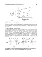
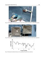
the real parts of impedance value (102.5 Ω) and the imaginary parts of impedance present
inductive characteristic (+41.3 Ω) at 900 MHz frequency. The inductive impedance can be
available for matching the capacitive RFID chip.


Fig. 9. Simulated and measured results of return loss spectrum


Fig. 10. Simulated results of impedance spectrum
The radiation patterns are obtained by an automatic measurement system in an anechoic
chamber. The under-tested antenna is located on the X-Y plane shown in Fig. 4, and the
feeding line is located along the X-axis. Thus, two radiation patterns with Y-Z cut and X-Z
cut are obtained.
Advanced Radio Frequency Identification Design and Applications

70
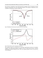
The two cut patterns with resonant 900 MHz are represented in Fig. 11 respectively.
Broadside patterns are observed in the Y-Z cut and quasi-omnidirectional patterns are
obtained in the X-Z cut. The measured maximum gain was 1.68 dBi for 900 MHz. For
polarizations, the AR spectrum is presented in Fig. 12. The minimum AR with 0.16 at
φ
=
0°,
θ
= 90°and the right-hand circular polarizations (–3dB AR BW = 383 MHz) are observed
along the direction of the
φ
and

θ
, thus the proposed antenna can be applied to circular
polarization applications which represents one of the availabilty and usefulness in contrast
to the conventional meander-line and meander-slot tags.


Fig. 11. Radiation patterns for 900 MHz


Fig. 12. AR spectrum
4. Conjugate matching performance
For example, the effective transmitted power
R
EIRP of reader is 1W, the sensitivity P
chip
of
tag microchip is -10dBm, the maximum tag antenna gain G = 1.62dBi, and the activation
An Inductive Self-complementary Hilbert-curve Antenna for UHF RFID Tags

71
distance d
min/max
= 2.5/3 m, the power transmission factor can be obtained
τ
= 0.73/0.87 by
using (2). Then, from (3) and tag antenna impedance (Z
A
= 102.5+j41.3
Ω
), the microchip

impedance (Z
chip
= 14.7-j45.2
Ω
) is calculated. For 900 MHz signal, the capacitance (757 pf)
of the chip microchip is presented.
For applications, the variation in antenna impedance, microchip impedance and tuning pad
(L
t
= 1.0, 2.0, 3.0, 4.0 and 5.0 mm) is shown in Table I. The varied inductive impedance can
be available for matching the related capacitive RFID chip (564–787 pf) by tuning the pad
length.


L
t
(mm)

Z
A
(Ω)

G
max

(dB)
d
min/max

(m)

τ
min/max
Z
chip
(Ω)

1 97.8+j46.3 0.98 2.5/3 0.71/0.96 15.6- j46.4
2 98.7+j45.6 1.12 2.5/3 0.68/0.99 14.3- j45.5
3 97.3+j44.2 1.21 2.5/3 0.78/0.98 15.7- j44.3
4 99.6+j43.4 1.38 2.5/3 0.76/0.93 14.2- j45.8
5 102.5+j41.3 1.62 2.5/3 0.73/0.87 14.7- j45.2
Table 1. Variation results
A microchip, RI-UHF-STRAP-08 of TI, is used for applications [43]. The data sheet is
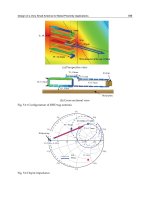
presented in Table 2. The diagram of complex plane
()Z
ω
is presented in Fig. 13. The
microchip impedance locus
()
chip
Z
ω
is firstly plotted in the complex plane. The arrowhead
attached to the locus indicates the direction of increasing
ω
from 860 to 960 MHz. Then,
tuning the length, as g=0.45 mm, L
f
= 5.8 mm and L
t

= 6.3 mm, the antenna impedance locus
()
a
Z
ω
is obtained.

The intersection of these two loci corresponds to the operating point. Due
to the operating point
chip
Z
= 287+j55
Ω
and
a
Z
= 287-j55
Ω
,
τ
=0.54 is calculated by (2). As
R
EIRP =1W, P
chip
= -13dBm and G = 1.62dBi,
max
d =33 m is obtained by (1).


Fig. 13. Impedance locus

Advanced Radio Frequency Identification Design and Applications

72
PART NUMBER RI-UHF-STRAP-08
Absolute Maximum Ratings
NOTES Min Max Unit
Input current, pad to pad

1 mA
Input voltage to any pad
(sustained)

1.5 V
Power dissipation TA = 25°C

1.5 mW
Single Strap -40 85
Storage temperature range
On Reel -40 45
°C
Read -40 65
Operating temperature
Write -25 65
°C
Assembly survival
temperature
1 minute maximum

150 °C
RF Exposure 800 ~ 1000 MHz

10 dBm
Charged-Device
Model (CDM)
0.5

kv
ESD immunity
Human-Body Model
(HBM)
2

kv
Recommended Operating Conditions

Min Max Unit
T
A
Operating temperature

-40 65 °C
f
res
Carrier frequency

860 960 MHz
Electrical Characteristics
PARAMETER TEST CONDITIONS Min/ Max Typ Unit
Reading -9/ - -13
Sensitivity

Programming -6/ - -19
dBm
∆ Change in modulator
reflection coefficient

>0.2

t
DRET
Data retention

10/ -

Years
W&E Write and erase
endurance

100000/ -

Cycles
Typical Read (–13 dB)

380 Ω
Strap Parallel Impedance

2.8 pF
Table 2. Specification of microchip RI-UHF-STRAP-08
For deterministic design, the design procedure is stated as: The guided wavelength (
/2g
λ

)
of the central frequency determines the total length of series Hilbert-curve. The desired
response and impedance are then tuned by L
t
. The final tuning is with g. Using (1) and (2)
with the specifications and boundary condition d
1/2
, the Z
chip
is obtained. If it is not satisfied,
retuning L
t
and g till the desired value is achieved.
5. Conclusion
The self-complementary antenna with Hilbert-curve configuration for RFID UHF-band tags
is presented in this paper. The good performance of compact, broadband (BW=150 MHz),
circular polarization and conjugate impedance matching are achieved for applications. The
An Inductive Self-complementary Hilbert-curve Antenna for UHF RFID Tags

73
structure is smaller in size and easy to fabricate in tag circuits. Its operations cover UHF-
bands 820 to 935 MHz for return loss
< -10dB. Both simulation and measurement results are
agreed with the verified frequency responses. The inductive impedance is achieved and be
available for matching the capacitive RFID chip.
In field analysis, broadside patterns are observed in the Y-Z cut and quasi-omnidirectional
patterns are obtained in the X-Z cut. The measured maximum gain was 1.68 dBi for 900
MHz. The circular polarization (–3dB AR BW = 383 MHz) feature of radiation patterns for
900 MHz are presented. It is a compact and available tag antenna for UHF RFID
applications.

6. References
[1] Marrocco, G. (2003). Gain-optimized self-resonant meander line antennas for RFID
applications. IEEE Antennas Wireless Propag. Lett., Vol. 2, pp. 302–305, ISSN: 1536-
1225.
[2] Keskilammi, M. & Kivikoski, M. (2004). Using text as a meander line for RFID
transponder antennas. IEEE Antennas Wireless Propag. Lett., Vol. 3, pp. 372–374,
ISSN: 1536-1225.
[3] Ukkonen, L.; Sydanheimo, L. & Kivikoski, M. (2005) Effects of metallic plate size on the
performance of microstrip patch-type tag antennas for passive RFID. IEEE Antennas
Wireless Propag. Lett., Vol. 4, pp. 410–413, ISSN: 1536-1225.
[4] Son, H.W. & Pyo, C.S. (2005). Design of RFID tag antennas using an inductively coupled
feed,” Electron. Lett., Vol. 41, No. 18, pp. 994–996, ISSN: 0013-5194.
[5] Rao, K.V.S.; Nikitin, P.V. & Lam, S.F. (2005). Antenna design for UHF RFID tags: a
review and a practical application. IEEE Trans. Antennas Propag., Vol. 53, No. 12, pp.
3870–3876, ISSN: 0018-926X.
[6] Ukkonen, L.; Schaffrath, M.; Engels, D.W.; Sydanheimo, L. & Kivikoski, M. (2006).
Operability of folded microstrip patch-type tag antenna in the UHF RFID bands
within 865-928 MHz. IEEE Antennas Wireless Propag. Lett., vol. 5, pp. 414–417, ISSN:
1536-1225.
[7] Chang, C.C. & Lo, Y.C. (2006). Broadband RFID tag antenna with capacitively coupled
structure,” Electron. Lett., Vol. 42, No. 23, pp. 1322–1323, ISSN: 0013-5194.
[8] Son, H.W.; Choi, G.Y. & Pyo, C.S. (2006). Design of wideband RFID tag antenna for
metallic surfaces. Electron. Lett., Vol. 42, No. 5, pp. 263–265, ISSN: 0013-5194.
[9] Ahn, J.; Jang, H.; Moon, H. Lee, J.W. & Lee, B. (2007). Inductively coupled compact RFID
tag antenna at 910 MHz with near-isotopic radar cross-section (RCS) patterns. IEEE
Antennas Wireless Propag. Lett., Vol. 6, pp. 518–520, ISSN: 1536-1225.
[10] Hu, S.; Law, C.L. & Dou, W. (2007). Petaloid antenna for passive UWB-RFID tags.
Electron. Lett., Vol. 43, No. 22, pp. 1174–1176, ISSN: 0013-5194.
[11] Vemagiri, J.; Balachandran, M.; Agarwal, M. & Varahramyan, K. (2007). Development of
compact half-sierpinski fractal antenna for RFID applications. Electron. Lett., Vol. 43,

No. 22, pp. 1168–1169, ISSN: 0013-5194.
[12] Kim, K.H.; Song, J.G.; Kim, D.H.; Hu, H.S. & Park, J.H. (2007). Fork-shaped RFID tag
antenna mountable on metallic surfaces. Electron. Lett., Vol. 43, No. 23, pp. 1400–
1402, ISSN: 0013-5194.
Advanced Radio Frequency Identification Design and Applications

74
[13] Olsson, T.; Hjelm, M.; Siden, J. & Nilsson, H.E. (2007). Comparative robustness study of
planar antenna. IET Microw. Antennas Propag., Vol. 1, No. 3, pp. 674–680, ISSN:
1751-8725.
[14] Marrocco, G. (2007). RFID antennas for the UHF remote monitoring of human subjects.
IEEE Trans. Antennas Propag., Vol. 55, No. 6, pp. 1862–1870, ISSN: 0018-926X.
[15] Calabrese, C. & Marrocco, G. (2008). Meandered-slot antennas for sensor-RFID tags.
IEEE Antennas Wireless Propag. Lett., Vol.7, pp. 5–8, ISSN: 1536-1225.
[16] Mushiake, Y. (1992). Self-complementary antennas. IEEE Antennas Propag. Mag., Vol. 34,
No. 6, pp. 23–29, ISSN: 1045-9243.
[17] Mushiake Y. (2004). A report on Japanese developments of antennas from yagi-uda
antenna to self-complementary antennas,”IEEE Antennas Propag. Mag., Vol. 46, No.
4, pp. 47–60, ISSN: 1045-9243.
[18] Xu, P.; Fujimoto, K. & Lin, S. (2002). Performance of quasi-self-complementary antenna
Using a monopole and a slot, Proceeding of IEEE Int. Symp. Antennas and Propag.,
pp. 464–477, ISBN: 0-7803-7330-8, San Antonio, Texas, June 2002, USA.
[19] Xu, P. & Fujimoto, K. (2003). L-shape self-complementary antenna, Proceeding of IEEE
Int. Symp. Antennas and Propag., pp. 95–98, ISBN: 0-7803-7846-6, Columbus, Ohio,
June 2003, USA.
[20] Mosallaei, H. & Sarabandi, K. (2004). A Compact Ultra-wideband Self-complementary
Antennas with Optimal Topology and Substrate, Proceeding of IEEE Int. Symp.
Antennas and Propag., pp. 1859–1862, ISBN: 0-7803-8302-8, Monterey, California
June 2004, USA.
[21] Saitou, A.; Iwaki, T.; Honjo, K.; Sato, K.; Koyama, T. & Watnabe, K. (2004). Practical

realization of self-complementary broadband antenna on low-loss resin substrate
for UWB applications, Proceeding of Int. IEEE MTT-S, Microw. Symp. Digest, pp.
1265–1268, ISBN: 0-7803-8331-1, YKC Corp., October 2004, Tokyo, Japan.
[22] Wong, K.L.; Wu, T.Y.; Su, S.W. & Lai, J.W. (2003). Broadband printed quasi-self-
complementary antenna for 5.2/5.8 GHz operation. Microwave Opt. Technol. Lett.,
Vol. 39. No. 6, pp. 495-496, ISSN: 1098-2760.
[23] Chen, W.S.; Chang, C.T. & Ku, K.Y. (2007). Printed triangular quasi-self-
complementary antennas for broadband operation, Proceeding of Int. Symp. Antennas
and Propag., pp. 262–265, Niigata University, August 2007, Niigata, Japan.
[24] Sagan, H. (1994). Space-filling curves, Springer-Verlag, ISBN: 3-540-94265-3, New York.
[25] Anguera, J.; Puente, C. & Soler, J. (2002). Miniature monopole antenna based on the
fractal Hilbert curve, Proceeding of IEEE Int. Symp. Antennas and Propag., Vol. 4, pp.
546–549, ISBN: 0-7803-7330-8, San Antonio, Texas, June 2002, USA.
[26] Best, S.R. & Morrow, J.D. (2002). The effectiveness of space-filling fractal geometry in
lowering resonant frequency. IEEE Antennas Wireless Propag. Lett., Vol. 1, pp. 112–
115, ISSN: 1536-1225.
[27] Gonzalez-Arbesu, J.M.; Blanck, S. & Romeu, J. (2003). The Hilbert curve as a small self-
resonant monopole from a practical point of view. Microwave Opt. Technol. Lett.,
Vol.39, No. 1, pp. 45–49, ISSN: 1098-2760.
[28] Yang, X.S.; Wang, B.Z. & Zhang, Y. (2006). Two-port reconfigurable Hilbert curve patch
antenna. Microwave Opt. Technol. Lett., Vol. 48, No. 1, pp. 91–93, Jan. 2006. ISSN:
1098-2760.
An Inductive Self-complementary Hilbert-curve Antenna for UHF RFID Tags

75
[29] Rathod, J.M. & Kosta, Y.P. (2009). Low cost development of RFID antenna, Proceeding of
Asia Pacific. Microwave Conference, Vol. 7, NO. 10, pp. 1060-1063, ISBN: 978-1-4244-
2801-4. Dec. 2009, Singapore.
[30] Toccafondi, A. & Braconi, P. (2007). Compact meander line antenna for HF-UHF tag
integration. Proceeding of IEEE Int. Symp. Antennas and Propag., Vol. 9, NO. 15, pp.

5483-5486 , ISBN: 978-1-4244-0877-1, June 2007, Hawaii.
[31] Kin, S.L.; Mun, L.N. & Cole, P.H. (2007). Miniaturization of Dual Frequency RFID
Antenna with High Frequency Ratio. Proceeding of IEEE Int. Symp. Antennas and
Propag., Vol. 9, No. 15, pp. 5475-5478 , ISBN: 978-1-4244-0877-1, June 2007, Hawaii.
[32] Roudet, F.; Vuong, T.P. & Tedjini, S. (2007). Metal effects over 13.56 MHz RFID reader
antenna in an electrical switchboard. Proceeding of IEEE Int. Symp. Antennas and
Propag., Vol. 9, NO. 15, pp. 2777-2780, ISBN: 978-1-4244-0877-1. June 2007, Hawaii.
[33] Pengcheng, L.; Yu, J.R. & Chieh, P.L. (2008). A experiment study of RFID antennas for
RF detection in liquid solutions. Proceeding of IEEE Int. Symp. Antennas and Propag.,
Vol. 5, NO. 11, pp. 1-4, ISBN: 978-1-4244-2041-4. July 2008, San Diego, CA.
[34] Toccafondi, A.; Giovampaola. C.D.; Mariottini, F. & Cucini, A. (2009). UHF-HF RFID
integrated tag for moving vehicle identification. Proceeding of IEEE Int. Symp.
Antennas and Propag., Vol. 1, NO. 5, pp. 1-4, ISBN: 978-1-4244-3647-7. June 2009,
Charleston, SC.
[35] Iliev, P.; Le Thuc, P.; Luxey, C. & Staraj, R. (2009). Dual-band HF-UHF RFID tag
antenna. Electron. Lett., Vol. 45, NO. 9, pp. 439-441, ISBN: 0013-5194.
[36] Hirvonen, M.; Pesonen, N.; Vermesan, O.; Rusu, C. & Enoksson, P. (2008). Multi-system,
multi-band RFID antenna: Bridging the gap between HF- and UHF-based RFID
applications. Proceeding of European Microwave Conference on Wireless Technol., Vol.
27, No. 28, pp. 346-349, ISBN: 978-2-87487-008-8. Oct. 2008, Amsterdam.
[37] Wang, D.; Xu, L.; Huang, H. & Sun, D. (2009). Optimization of Tag Antenna for RFID
System. Proceeding of Information Technology and Computer Science on International
Conference, Vol. 2, No. 26, pp. 36-39, ISBN: 978-0-7695-3688-0. July 2009, Kiev.
[38] Bassen, H.; Seidman, S.; Rogul, J.; Desta, A. & Wolfgang, S. (2007). An Exposure System
for Evaluating Possible Effects of RFID on Various Formulations of Drug Products.
Proceeding of IEEE Int. Conference on RFID, Vol. 26, NO 28, pp. 191-198, ISBN: 1-
4244-1013-4. March 2007, Grapevine, TX.
[39] Allen, M.L.; Jaakkola, K.; Nummila, K. & Seppa, H. (2009). Applicability of Metallic
Nanoparticle Inks in RFID Applications. IEEE Trans. Components and Packaging
Technologies, Vol. 32, No. 2, pp. 325-332, ISBN: 1521-3331.

[40] Mayer, L.W. & Scholtz, A.L. (2008). A Dual-Band HF / UHF Antenna for RFID Tags.
Proceeding of IEEE 68th Vehicular Technology Conference, Vol. 21, No. 24, pp. 1-5,
ISBN: 1090-3038. Sept. 2008, Calgary, BC.
[41] Kariyapperuma, A.V. & Dayawansa, I.J. (2009). Bi-loop’ RFID reader antenna for
tracking fast moving tags. Proceeding of IEEE Radio and Wireless Symposium, Vol. 18,
No. 22, pp. 449-452, ISBN: 978-1-4244-2698-0. Jan. 2009, San Diego, CA. HFSS
version 11.0, Ansoft Software Inc., 2007. Texas Instruments Incorporated,
/>.
[42] Vinoy, K.J.; Jose, K.A.; Varadan, V.K. & Varadan, V.V. (2001). Resonant Frequency of
Hilbert Curve Fractal Antennas. Proceeding of IEEE Int. Symp. Antennas and Propag.,
Vol. 3, pp. 648–4651, ISBN: 0-7803-7070-8. July 2001Boston, MA.
Advanced Radio Frequency Identification Design and Applications

76
[43] Vinoy, K.J.; Jose, K.A.; Varadan, V.K. & Varadan, V.V. (2001) Hilbert Curve Fractal
Antennas with Reconfigurable Characteristics. Inte. Microwave Symposium Digest,
IEEE MTT-S l. Vol.1, pp.381-384, ISBN: 0-7803-6538-0. 2001, Phoenix, AZ.
[44] Yang, X.S.; Wang, B.Z. & Zhang, Y. (2005). A Reconfigurable Hilbert Curve Patch
Antenna. Proceeding of IEEE Int. Symp. Antennas and Propag., Vol.2B, pp.613-616,
ISBN: 0-7803-8883-6. July 2005.
[45] Murad, N.A.; Esa, M.; Yusoff, M.F.M.; & Ali, S.H.A. (2006). Hilbert Curve Fractal
Antenna for RFID Application. Inte. RF and Microwave Conference, pp.182-186, ISBN:
0-7803-9745-2. Sept. 2006, Putra Jaya.
[46] Takemura, N. (2009). Inverted-FL antenna with self-complementary structure. IEEE
Trans. Antennas Propag., Vol. 57, No.10 , pp. 3029–3034, ISSN : 0018-926X.
[47] Suh, S.Y.; Nair, V.K.; Souza, D. & Gupta, S. (2007). High isolation antenna for multi-
radio antenna system using a complementary antenna pair. Proceeding of IEEE Int.
Symp. Antennas and Propag., pp.1229-1232, ISBN: 978-1-4244-0877-1. June 2007,
Honolulu, HI.
[48] Guo, L.; Chen, X. & Parini, C.G. (2008). A Printed Quasi-Self-Complementary Antenna

for UWB Applications. Proceeding of IEEE Int. Symp. Antennas and Propag., pp.1-4,
ISBN: 978-1-4244-2041-4. July 2008, San Diego, CA.
[49] Guo, L.; Wang, S.; Chen, X. & Parini, C. (2009). A Small Printed Quasi-Self-
Complementary Antenna for Ultrawideband Systems. IEEE Antennas Wireless
Propag. Vol.8, 2009, pp.554-557, ISSN : 1536-1225.
[50] Xu, P.; Kyohei F. & Shiming L. (2002). Performance of Quasi-Selfcomplementary
Antenna Using a Monopole and a Slot. Proceeding of IEEE Int. Symp. Antennas and
Propag., pp.464-467, ISBN: 0-7803-7330-8. 2002.

5
Design of a Very Small Antenna for
Metal-Proximity Applications
Yoshihide Yamada
National Defence Academy, Dept. of Electronic Engineering
Japan
1. Introduction
A radio frequency identification (RFID) system consists of a reader, a writer, and a tag. Film-
type half-wavelength dipole antennas (shown in Fig. 1.1) have been used as tag antennas in
many applications [1]. The antenna performance is governed by the electric current in the
tag. When the abovementioned antenna is mounted on the surface of a metallic object, the
radiation characteristics are seriously degraded because of the image current induced in the
object. Therefore, studies have been carried out to construct tag antennas that are suitable
for use with metallic objects, and some promising antenna types have been proposed.
In this chapter, design approaches for metal-proximity antennas (antennas placed in close
proximity to a metal plate) are discussed. In Section 2, typical metal-proximity antennas are
described. An example of the aforementioned type of antenna is a normal-mode helical
antenna (NMHA), which can show high efficiency despite its small size. We focus on the
design of this antenna. In Section 3, the fundamental equations used in the NMHA design
are summarized. In particular, we propose an important equation for determining the self-
resonant structure of the antenna. We fabricate an antenna to show that its electrical

characteristics are realistic. In Section 4, we explain the impedance-matching method
necessary for the NMHA and provide a detailed description of the tap feed. In Section 5, we
discuss the use of NMHA as a tag antenna and provide the read ranges achieved.

Electric current
IC chip
28mm
94mm
Electric current

Fig. 1.1 A typical tag antenna
2. Tag antennas for metal-proximity use
Typical examples of metal-proximity tag antennas are given in Table 2.1. Some examples of
metal-proximity antennas are patch antennas [2] and slot antennas [3], which can be
Advanced Radio Frequency Identification Design and Applications

78
mounted on a metal plate. Since these antennas comprise flat plates, the antenna thickness
decreases but the size does not small. Another example of a metal-proximity antenna is the
normal-mode helical antenna (NMHA) [4]. The wire length of this antenna is approximately
one-half of the wavelength, and hence, the antenna is small-sized. Moreover, because this
antenna has a magnetic current source, it can be mounted on a metallic plate. The antenna
gain increases when the antenna is placed in the vicinity of a metal plate. Because the
antenna input resistance is small, a tap-feed structure is necessary to increase the resistance.

・Frequency ：953MHz
・Thickness : 4mm
・Read range ：13m
・Commercial products
・Frequency ：915MHz

・Thickness : 0.25mm
・Read range ：5m
・Researching
・Frequency ：953MHz
・Thickness : 16mm
・Read range ：8m
・Researching
[2] Patch antenna [3] Slot antenna
[4] Normal mode helical
antenna
76mm
76mm
16mm
20mm
80mm
30mm
Ta pIC chip
IC chip
IC chip
11mm

Table 2.1 Metal-proximity tag antennas

receiving a ntenna
small transmitter
(tire pressure sensor)
receiver unit
air pressure data
(315MHz)

Fig. 2.1 Application of NMHA to tire-pressure monitoring system
The feasibility of using very small NMHAs in a tire-pressure monitoring system (TPMS) [5]
and metal-proximity RFID tags [6] has been studied. The RFID applications are explained in
Design of a Very Small Antenna for Metal-Proximity Applications

79
detail in Section 5. Figure 2.1 shows the TPMS system (called AIRwatch) developed by The
Yokohama Rubber Co., Ltd. Transmitters connected to tire-pressure sensors are mounted on
the wheels, and a receiver unit is placed on the dashboard. A receiving antenna (a film
antenna) is attached to the windshield. Each sensor uses the FSK scheme to modulate 315-
MHz continuous waves with air pressure data. The modulated waves are transmitted from
a small loop antenna in the sensor. The receiving antenna collects all the transmitted waves,
and the pressure levels are indicated on the receiver unit. To apply this system to trucks and
buses, it is necessary to replace the small-loop antenna with an NMHA [7] since the gain and
effectiveness of the latter are high under metal-proximity conditions.
3. Design and electrical characteristics of normal-mode helical antenna
3.1 Features of NMHA
The structural parameters of the NMHA are shown in Fig. 3.1. The length, diameter, and
number of turns of the antenna are denoted by H, D, and N, respectively. The diameter of
the antenna wire is denoted by d. A comprehensive treatment of this antenna has been given
by Kraus [8]. In Kraus’s study, the antenna current was divided across the straight part and
circular parts of the antenna. Conceptual expressions for the two current sources are shown
in Fig. 3.1. The straight part acts like a small dipole antenna, and the circular parts act like
small loop antennas. The radiation characteristics of these small loops are equivalent to
those of a small magnetic current source. Therefore, the radiated electric fields are composed
of two orthogonal electrical components produced by electric and magnetic current sources.
Hence, the radiated electric field polarization becomes circular or elliptical depending on the
H-to-D ratio. Because the radiated fields are produced by small electrical and magnetic
current sources, the radiation patterns are almost constant for various small antennas. The
directional gain is almost 1.5 (1.8 dBi).

D
D
small dipole small loop
Electric current source
+
H
N
I
I
J
N=10
d
R
rD
-jX
D
R
rL
+jX
L
Magnetic current source

Fig. 3.1 Conceptual equivalence of normal-mode helical antenna
Advanced Radio Frequency Identification Design and Applications

80
The existence of a magnetic current source is advantageous for using an antenna in the
proximity of a metal plate. The electrical image theory indicates that radiation from a
magnetic current source is increased by the existence of a metal plate. Another important

feature of an NMHA is its impedance. A small dipole has capacitive reactance, and the small
loops have inductive reactance. By appropriate choice of the H, D, and N values, the
capacitive and inductive reactances can be made to cancel out each other. This condition is
called the self-resonant condition, and it is important for efficient radiation production. In
this case, the input impedance becomes a pure resistance. It should be noted that this pure
resistance is small, and therefore, an impedance-matching structure is necessary. Moreover,
the ohmic resistance of the antenna wire must be reduced to a considerable extent.
Important aspects of the NMHA design are summarized in Table 3.1. Simple equations for
R
r
, R
l
, E
θ
, and E
φ
, which are related to radiation production, have been presented by Kraus
[8]. A useful expression for the inductive reactance (X
L
) has been developed by Wheeler [9].
However, a correct expression for the capacitive reactance (X
C
) has not yet been presented;
we plan to develop the appropriate equation for this value. We also compare the theoretical
values of the antenna quality factor (Q) with the experimental results. We then consider an
important design equation that can be used to determine the self-resonant structures. This
equation is derived from the equations for X
L
and X
C

, and its accuracy is confirmed by
comparison of the calculated and simulated results. Using these equations, we can design
small antennas with high gain. Because the radiation patterns are almost constant, the
antenna efficiency is important for achieving high gain. Finally, the impedance-matching
method is important, and three methods are usually considered. However, in the first
method among these, the circuit method, the antenna gain is greatly reduced because of the
accompanying ohmic resistances of the circuit elements.

Aspect Features Comments
Equations of electrical
characteristics
Input resistance: R
r
, R
l

Radiation fields: E
θ
, E
φ

Input reactance: X
L
, X
C

Q factor
Antenna efficiency
Polarization
Self-resonance

Bandwidth
Self-resonant structure Determine relation between N,
H, D: Using X
L
= X
C
condition
Design equation must
be developed
Design data for high
antenna performance
Antenna efficiency

Low ohmic resistance is
necessary
Impedance matching Circuit method
Off-center feed
Tap feed
Not suitable
Limited application
Most useful
Table 3.1 Important aspects of NMHA design
To estimate the electrical characteristics of the NMHA, we perform electromagnetic
simulations based on the method of moments (MoM) using a commercial simulator, FEKO.
Design of a Very Small Antenna for Metal-Proximity Applications

81
We compare the simulated results with the experimental results. By appropriate choice of
the simulation parameters, we can obtain reliable results.
3.2 Equations for main electrical characteristics

3.2.1 Equations of electrical constants for radiation
The radiation characteristics of small antennas are estimated from the antenna input
impedance, which is given by
Zin = R
rD
+ R
rL
+ R
l
+ j(X
L
-X
C
) (3.1)
Here, R
rD
is the radiation resistance of the small dipole; R
rL
, the radiation resistance of the
small loops; and R
l
, the ohmic resistance of the antenna wire. X
L
and X
C
are the inductive
and capacitive reactances, respectively. The exact expressions for X
L
and X
C

will be
discussed in the later sections.
We now summarize the expressions for the radiation characteristics.
a. Small dipole [10]
The radiation characteristics of the small dipole are given by the following expressions, in
which the structural parameters shown in Fig. 3.1 are used:

2
2
20
D
H
Rr
π
λ
⎛⎞
=
⎜⎟
⎝⎠
(3.2)
Here, λ is the wavelength.

π
2
2
3
I1
Esin
j 4
j

R
j
He
RR
R
κ
θ
κ
κ
θ
ωε
−
⎛⎞
=+−
⎜⎟
⎝⎠
(3.3)
Here, I is the antenna current, R is the distance from the antenna, and k is the wave number.
The terms 1/R
2
and 1/R
3
represent the static electric field and the inductive electric field,
respectively. The values of 1/R
2
and 1/R
3
decrease rapidly as R increases. The 1/R term
indicates the far electric field and corresponds to the radiated electric field.
b.

Small loop [11]
The radiation characteristics of the small loops are given by the following expressions, in
which the structural parameters shown in Fig. 3.1 are used:
R
rL
= 320π
6
(a/λ)
4
n
2
(3.4)
Here, a and n indicate the radius of the loop and the number of turns, respectively.

μ
π
2
j
I
Esin
4
jR
Se
R
R
κ
φ
ωκ
θ
−

⎛⎞
=−+
⎜⎟
⎝⎠
(3.5)
The 1/R term represents the radiated electric field. Here, I is the loop antenna current, and S
is the area of a loop.
3.2.2 Equations for input reactance of NMHA [12]
The equivalent model of the small dipole and small loops (shown in Fig. 3.1) cannot be used
for the expressions for X
L
and X
C
. For the stored electromagnetic power of the NMHA,
highly precise electromagnetic models must be developed.
Advanced Radio Frequency Identification Design and Applications

82
a. Self-resonant structure
The self-resonant structures of an NMHA are important when designing reactance
equations. These structures can be obtained from the structural parameters that satisfy the
condition X
L
= X
C
. The aforesaid parameters can be easily identified by electromagnetic
simulations, but such simulations are tedious and time-consuming An alternative method
would involve the use of design equations. However, a convenient equation for determining
the resonant structure has not yet been developed; we plan to develop such an equation.
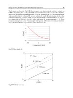
The self-resonant structures calculated from simulations are shown in Fig. 3.2. Here, the

315-MHz data used for the TPMS are shown. For a given N value, a strict relationship
between H and D is determined. As N increases, D decreases rapidly, indicating that the
total wire length (L
0
) of the antenna changes only to a slight extent. The calculated wire
lengths are shown in Fig. 3.3. The values of L
0
/λ range from 0.35 to 0.72. These data are
important for choosing the appropriate wire length when fabricating an actual antenna.61.38

0.02 0.04 0.06 0.08 0.10
0.005
0.010
0.015
0.020
0.025
0.030
0.035
D [m]
H [m]
N = 15
N = 10
N = 5
f = 315 MHz
λ
= 0.95 m
d = 0.55 mm

Fig. 3.2 NMHA resonant structures

0.00 0.02 0.04 0.06 0.08 0.10
0.3
0.4
0.5
0.6
0.7
L
0
/
λ
H/
λ
f = 315 MHz
d = 0.55 mm
N=5
N=10
N=15

Fig. 3.3 NMHA wire lengths (L
0
)
Design of a Very Small Antenna for Metal-Proximity Applications

83
The typical electrical performance of the self-resonant structure is the excited current in the
antenna. The peak electrical currents of the resonance are shown in Fig. 3.4. To illustrate the
physical phenomena in detail, sequential N values of 4, 5, and 6 are selected. In the
calculation, the feed voltage V is set to 1 V. The current values show a peak near the
resonant structures. The current decreases rapidly with an increase in the distance between

the resonant structure and the measurement point. The condition X
L
= X
C
is important for
the production of strong radiation currents. Another important point to be noted is that the
peak current values are almost inversely proportional to H. Since V = R
in
I
M
, an increase in I
M

implies a decrease R
in
. As exepected, R
in
decreases as H decreases.

0.02
0.04
0.06
0.08
0.10
0.0
0.5
1.0
1.5
0.02
0.03

0.04
I
M
[
A]
D

[
m
]
H

[
m]
N = 6
N = 5
N = 4
V = 1 [V]

Fig. 3.4 Maximum currents near the resonances
b. Equation for inductive reactance
The calculated magnetic field distributions are shown in Fig. 3.5. It can be seen that the
magnetic field vectors constantly pass through the coil. The field distributions around the
anntena are similar to those in the case of a conventional coil. No unique distributions are
observed.
The equation for the antenna inductance (L
W
) was established by Wheeler [9]. By applying
Wheeler’s equation to the center-feed antenna, we obtain

[]
2
6
19.7
10 H
920
W
ND
L
DH
−
=×
+
(3.6)
Here, the unit [H] stands for Henry.
The inductive reactance (X
L
) is given by

[
]

LW
XL
ω
=
Ω (3.7)
The calculated inductive reactance X
L
(Fig. 3.6) is rather large: it ranges from 59 Ω to 205 Ω.

In this figure, the dependence of X
L
on the structural parameters (N, D, and H) is explained
by taking into account Eq. (3.6). The relation between X
L
and H is determined on the basis of
Advanced Radio Frequency Identification Design and Applications

84
the denominator in Eq. (3.6). The change in X
L
with N is rather slow and is determined by
the term ND
2
in this equation.

～
I
M
H
D
H

Fig. 3.5 Magnetic field distribution

0.02 0.04 0.06 0.08 0.10
50
100
150
200

X
L
[Ω]
H
[m]
N = 15
N = 10
N = 5

Fig. 3.6 Inductive reactance
c. Equation for capacitive reactance
In this chapter, we discuss the development of a useful expression for capacitive reactance.
The calculated electric field distributions are shown in Fig. 3.7. The directions of the electric
field vectors appear to be unique. At the edges of the antenna, the vectors appear to
converge or diverge in specific areas. These areas form short cylinders of height αH, as
shown by the dashed lines.
Design of a Very Small Antenna for Metal-Proximity Applications

85
+Q
-Q
I
M
E
S
E
L
E
U
D

H
αH
αH
E

Fig. 3.7 Electric field distributions

0.02 0.04 0.06 0.08 0.10
0
100
200
300
400
Q
E
[pC]
H [m]
N = 4
N = 6

Fig. 3.8 Stored charge
By applying the divergence theorem of Maxwell’s equation, we calculate the charge stored
in a cylinder from the following equation:

{
}
[]
C
SLU
Q EdS E dS E dS E dS

εε
== ++
∫∫ ∫∫ ∫∫ ∫∫
(3.8)
Here, the unit [C] stands for Coulomb. Surface integrals over the side wall, lower disc, and
upper disc of the cylinder are evaluated.
The calculated Q values are shown in Fig. 3.8. By comparing the cylinder height coefficients
(α) of many resonant structures, we estimated the value of α in the present study to be 0.21.
Advanced Radio Frequency Identification Design and Applications

86
The Q values are inversely proportional to H; this trend agrees well with the relationship
between I
M
and H shown in Fig. 3.4. This agreement corresponds to the relation Q = I
M
/ω.
The magnitude of ω (= 2πf) is 2 × 10
9
. If we set I
M
and H to 1.2 A and 0.02 m, respectively, in
Fig. 3.4, we have
I
M
/ω = 1.2/(2 × 10
9
) = 600 × 10
-12
(3.9)

The value derived using Eq. (3.9) corresponds well with the Q and H values (400 pC and
0.02 m, respectively) determined from Fig. 3.8. Thus, the use of Eq. (3.8) is justified.
The next step is to derive an expression for the capacitance (C) on the basis of Eq. (3.8). The
relationship between Q and C depends on the electric power (We). Two expressions for We
are given as follows.

2
2
e
Q
W
C
= (3.10)
This expression gives the total electric power stored in the +Q and –Q capacitor.


2
/2
eL
WEdv
ζε
=
∫∫∫
(3.11)
The volume integral gives the electric power in the NMHA. The coefficient ζ is introduced
to express the total power.
By equating Eqs. (3.10) and (3.11), we obtain an expression for C:

{
}

2
2
L
EdS
C
Edv
ε
ζε
=
∫∫
∫
∫∫
(3.12)
Eq. (3.12) can be converted into an expression based on the structural parameters:


2
22
2
22
()( )
3.82 (4.4 )
2
4(1 2)
()(12)
2
SUL
L
D
NDaHE E E

NHD
C
D
H
EH
επ π
επ α
ζα
ζε π α
⎧⎫
++
⎨⎬
+
⎩⎭
==
−
−
(3.13)
Here, we use the conditions E
S
= 1.1(E
L
+ E
U
) and E
S
= 2.15E
L
, on the basis of the simulation
results;

α
is the cylinder height shown in Fig. 3.7. For the N dependence, we recall the ND
2

term in Eq. (3.6). To model the gradual change of C with N we multiply N by (4.4aH+D)
2
.
The expression for X
C
is obtained from Eq. (3.13):


22
1 4 (1 2 ) 279
3.82 (4.4 ) (0.92 )
C
HH
X
C
NHD NHD
ζα λ
ω
ωεπ α π
−
== =
++
(3.14)
Here, we use ωε = 1/(60λ) and
α
= 0.21. Moreover, we set ζ to 7.66 for equating X

C
with X
L
at
N = 10; see Fig. 3.6.
The calculated X
C
values are shown in Fig. 3.9. At N = 10, the X
C
= X
L
condition is achieved
(Figs. 3.9 and 3.6). At N = 5 and N = 15, X
C
and X
L
are in good agreement with each other.
As a fall, agreement of X
C
and X
L
are well. Thus, Eq. (3.14) is confirmed to be useful.
Design of a Very Small Antenna for Metal-Proximity Applications

87
0.02 0.04 0.06 0.08 0.10
50
100
150
200

X
C
[Ω]
H [m]
N = 15
N = 10
N = 5

Fig. 3.9 Capacitive reactance

0.02 0.04 0.06 0.08 0.10
0.005
0.010
0.015
0.020
0.025
0.030
0.035
D/
λ
H/
λ
N = 5
N = 10
N = 15
Sim.
Eq. (3.16)

Fig. 3.10 Calculated and simulated self-resonant structures
3.2.3 Design equation for self-resonant structures [12]

The deterministic equation is given by equating Eqs. (3.7) and (3.14). The resulting equation
is

2
6
2
19.7 279
10
920
(0.92 )
ND H
DH
NHD
λ
ω
π
−
×=
+
+
(3.15)
To clarify the frequency dependence, we divide the numerator and denominator of Eq.
(3.15) by λ
2
and obtain
Advanced Radio Frequency Identification Design and Applications

88

2

2
19.7 ( ) 279
600
920 (0.92 )
DH
N
DH HD
N
λλ
π
π
λ
λλλ
=
++
(3.16)
An important feature of this design equation is that it becomes frequency-independent
when the structural parameters are normalized by the wavelength.
To ensure the accuracy of this equation, the calculated results are compared with the curves
in Fig. 3.2. Figure 3.10 shows this comparison. At N = 10, the curve obtained on the basis of
Eq. (3.16) agrees well with that obtained on the basis of the simulation results. At N = 5 and
N = 15, small differences are observed between the two curves; however, the maximum
difference is less than 9.4%. Thus, Eq. (3.16) is confirmed to be useful.
3.2.4 Ohmic resistance

L

W

ｔ

δ


Fig. 3.11 Cross-sectional view of antenna wire
Figure 3.11 shows a cross-sectional view of the antenna wire. The parameters W, t, and L
represent the width, thickness, and total length of the wire, respectively, and δ is the skin
depth:

2
δ
ω
μσ
= (3.17)
Here, σ is the conductance of the wire metal.
If the current is concentrated within the skin depth δ, the ohmic resistance is

()
11
2
l
LL
R
tW d
αα
δ
σδπσ
=
⋅= ⋅
+

(3.18)
Here, α is the coefficient of the tapered current distribution, and d is the wire diameter.
By applying Eq. (3.17) to Eq. (3.18), we obtain the following expression for the ohmic
resistance:

() ()
2
240 30 120
22
l
LLL
R
tW tW d
ππ
ααα
λ
σλσλσ
===
++
(3.19)
In small NMHAs, because the current distribution becomes sinusoidal, Eq. (3.19) agrees well
with the simulation result at α = 0.6.