HANDBOOK OFINTEGRAL EQUATIONS phần 8 docx

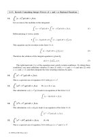
Example 1. Let us solve the integral equation
y(x) – λ

1
0
xty(t) dt = f(x), 0 ≤ x ≤ 1,
by the method of successive approximations. Here we have K(x, t)=xt, a = 0, and b = 1. We successively define
K
1
(x, t)=xt, K
2
(x, t)=

1
0
(xz)(zt) dz =
xt
3
, K
3
(x, t)=
1
3

1
0
(xz)(zt) dz =
xt
3
2
, , K

n
(x, t)=
xt
3
n–1
.
According to formula (5) for the resolvent, we obtain
R(x, t; λ)=
∞

n=1
λ
n–1
K
n
(x, t)=xt
∞

n=1

λ
3

n–1
=
3xt
3 – λ
,
where |λ| < 3, and it follows from formula (7) that the solution of the integral equation can be rewritten in the form
y(x)=f(x)+λ


1
0
3xt
3 – λ
f(t) dt,0≤ x ≤ 1, λ ≠ 3.
In particular, for f (x)=x we obtain
y(x)=
3x
3 – λ
,0≤ x ≤ 1, λ ≠ 3.
11.3-4. Orthogonal Kernels
For some Fredholm equations, the Neumann series (5) for the resolvent is convergent for all values
of λ. Let us establish this fact.
Assume that two kernels K(x, t) and L(x, t) are given. These kernels are said to be orthogonal
if the following two conditions hold:

b
a
K(x, z)L(z, t) dz =0,

b
a
L(x, z)K(z, t) dz = 0 (8)
for all admissible values of x and t.
There exist kernels that are orthogonal to themselves. For these kernels we have K
2
(x, t) ≡ 0,
where K
2

(x, t) is the second iterated kernel. It is clear that in this case all the subsequent iterated
kernels also vanish, and the resolvent coincides with the kernel K(x, t).
Example 2. Let us find the resolvent of the kernel K(x, t) = sin(x – 2t), 0 ≤ x ≤ 2π,0≤ t ≤ 2π.
We have

2π
0
sin(x – 2z) sin(z – 2t) dz =
1
2

2π
0
[cos(x +2t – 3z) – cos(x – 2t – z)] dz =
=
1
2

–
1
3
sin(x +2t – 3z) + sin(x – 2t – z)

z=2π
z=0
=0.
Thus, in this case the resolvent of the kernel is equal to the kernel itself:
R(x, t; λ) ≡ sin(x – 2t),
so that the Neumann series (6) consists of a single term and clearly converges for any λ.
Remark 2. If the kernels M

(1)
(x, t), , M
(n)
(x, t) are pairwise orthogonal, then the resolvent
corresponding to the sum
K(x, t)=
n

m=1
M
(m)
(x, t)
is equal to the sum of the resolvents corresponding to each of the summands.
•
References for Section 11.3: S. G. Mikhlin (1960), M. L. Krasnov, A. I. Kiselev, and G. I. Makarenko (1971),
J. A. Cochran (1972), V. I. Smirnov (1974), A. J. Jerry (1985).
Page 535
© 1998 by CRC Press LLC
© 1998 by CRC Press LLC
11.4. Method of Fredholm Determinants
11.4-1. A Formula for the Resolvent
A solution of the Fredholm equation of the second kind
y(x) – λ

b
a
K(x, t)y(t) dt = f(x), a ≤ x ≤ b, (1)
is given by the formula
y(x)=f(x)+λ


b
a
R(x, t; λ)f(t) dt, a ≤ x ≤ b, (2)
where the resolvent R(x, t; λ)isdefined by the relation
R(x, t; λ)=
D(x, t; λ)
D(λ)
, D(λ) ≠ 0. (3)
Here D(x, t; λ) and D(λ) are power series in λ,
D(x, t; λ)=
∞

n=0
(–1)
n
n!
A
n
(x, t)λ
n
, D(λ)=
∞

n=0
(–1)
n
n!
B
n
λ

n
, (4)
with coefficients defined by the formulas
A
0
(x, t)=K(x, t), A
n
(x, t)=

b
a
···

b
a
  
n








K(x, t) K(x, t
1
) ··· K(x, t
n
)

K(t
1
, t) K(t
1
, t
1
) ··· K(t
1
, t
n
)
.
.
.
.
.
.
.
.
.
.
.
.
K(t
n
, t) K(t
n
, t
1
) ··· K(t

n
, t
n
)








dt
1
dt
n
, (5)
B
0
=1, B
n
=

b
a
···

b
a
  

n








K(t
1
, t
1
) K(t
1
, t
2
) ··· K(t
1
, t
n
)
K(t
2
, t
1
) K(t
2
, t
2

) ··· K(t
2
, t
n
)
.
.
.
.
.
.
.
.
.
.
.
.
K(t
n
, t
1
) K(t
n
, t
2
) ··· K(t
n
, t
n
)









dt
1
dt
n
; n =0,1,2, (6)
The function D(x, t; λ) is called the Fredholm minor and D(λ) the Fredholm determinant. The
series (4) converge for all values of λ and hence define entire analytic functions of λ. The resolvent
R(x, t; λ) is an analytic function of λ everywhere except for the values of λ that are roots of D(λ).
These roots coincide with the characteristic values of the equation and are poles of the resolvent
R(x, t; λ).
Example 1. Consider the integral equation
y(x) – λ

1
0
xe
t
y(t) dt = f(x), 0 ≤ x ≤ 1, λ ≠ 1.
We have
A
0
(x, t)=xe

t
, A
1
(x, t)=

1
0




xe
t
xe
t
1
t
1
e
t
t
1
e
t
1




dt

1
=0, A
2
(x, t)=

1
0

1
0






xe
t
xe
t
1
xe
t
2
t
1
e
t
t
1

e
t
1
t
1
e
t
2
t
2
e
t
t
2
e
t
1
t
2
e
t
2






dt
1

dt
2
=0,
since the determinants in the integrand are zero. It is clear that the relation A
n
(x, t) = 0 holds for the subsequent coefficients.
Let us find the coefficients B
n
:
B
1
=

1
0
K(t
1
, t
1
) dt
1
=

1
0
t
1
e
t
1

dt
1
=1, B
2
=

1
0

1
0




t
1
e
t
1
t
1
e
t
2
t
2
e
t
1

t
2
e
t
2




dt
1
dt
2
=0.
Page 536
© 1998 by CRC Press LLC
© 1998 by CRC Press LLC
It is clear that B
n
= 0 for all subsequent coefficients as well.
According to formulas (4), we have
D(x, t; λ)=K(x, t)=xe
t
; D(λ)=1– λ.
Thus,
R(x, t; λ)=
D(x, t; λ)
D(λ)
=
xe

t
1 – λ
,
and the solution of the equation can be represented in the form
y(x)=f(x)+λ

1
0
xe
t
1 – λ
f(t) dt,0≤ x ≤ 1, λ ≠ 1.
In particular, for f (x)=e
–x
we obtain
y(x)=e
–x
+
λ
1 – λ
x,0≤ x ≤ 1, λ ≠ 1.
11.4-2. Recurrent Relations
In practice, the calculation of the coefficients A
n
(x, t) and B
n
of the series (4) by means of
formulas (5) and (6) is seldom possible. However, formulas (5) and (6) imply the following
recurrent relations:
A

n
(x, t)=B
n
K(x, t) – n

b
a
K(x, s )A
n–1
(s, t) ds, (7)
B
n
=

b
a
A
n–1
(s, s) ds. (8)
Example 2. Let us use formulas (7) and (8) to find the resolvent of the kernel K(x, t)=x – 2t, where 0 ≤ x ≤ 1 and
0 ≤ t ≤ 1.
Indeed, we have B
0
= 1 and A
0
(x, t)=x – 2t. Applying formula (8), we see that
B
1
=


1
0
(–s) ds = –
1
2
.
Formula (7) implies the relation
A
1
(x, t)=–
x – 2t
2
–

1
0
(x – 2s)(s – 2t) ds = –x – t +2xt +
2
3
.
Furthermore, we have
B
2
=

1
0

–2s +2s
2

+
2
3

ds =
1
3
,
A
2
(x, t)=
x – 2t
3
– 2

1
0
(x – 2s)

–s – t +2st +
2
3

ds =0,
B
3
= B
4
= ···=0, A
3

(x, t)=A
4
(x, t)=···=0.
Hence,
D(λ)=1+
1
2
λ +
1
6
λ
2
; D(x, t; λ)=x – 2t + λ

x + t – 2xt –
2
3

.
The resolvent has the form
R(x, t; λ)=
x – 2t + λ

x + t – 2xt –
2
3

1+
1
2

λ +
1
6
λ
2
.
• References for Section 11.4: S. G. Mikhlin (1960), M. L. Krasnov, A. I. Kiselev, and G. I. Makarenko (1971),
V. I. Smirnov (1974).
Page 537
© 1998 by CRC Press LLC
© 1998 by CRC Press LLC
11.5. Fredholm Theorems and the Fredholm Alternative
11.5-1. Fredholm Theorems
THEOREM 1.
If
λ
is a regular value, then both the Fredholm integral equation of the second kind
and the transposed equation are solvable for any right-hand side, and both the equations have unique
solutions. The corresponding homogeneous equations have only the trivial solutions.
THEOREM 2.
For the nonhomogeneous integral equation to be solvable, it is necessary and
sufficient that the right-hand side
f(x)
satisfies the conditions

b
a
f(x)ψ
k
(x) dx =0, k =1, , n,

where
ψ
k
(x)
is a complete set of linearly independent solutions of the corresponding transposed
homogeneous equation.
THEOREM 3.
If
λ
is a characteristic value, then both the homogeneous integral equation and the
transposed homogeneous equation have nontrivial solutions. The number of linearly independent
solutions of the homogeneous integral equation is finite and is equal to the number of linearly
independent solutions of the transposed homogeneous equation.
THEOREM 4.
A Fredholm equation of the second kind has at most countably many characteristic
values, whose only possible accumulation point is the point at infinity.
11.5-2. The Fredholm Alternative
The Fredholm theorems imply the so-called Fredholm alternative, which is most frequently used in
the investigation of integral equations.
T
HE FREDHOLM ALTERNATIVE.
Either the nonhomogeneous equation is solvable for any right-
hand side or the corresponding homogeneous equation has nontrivial solutions.
The first part of the alternative holds if the given value of the parameter is regular and the second
if it is characteristic.
Remark. The Fredholm theory is also valid for integral equations of the second kind with weak
singularity.
•
References for Section 11.5: S. G. Mikhlin (1960), M. L. Krasnov, A. I. Kiselev, and G. I. Makarenko (1971),
J. A. Cochran (1972), V. I. Smirnov (1974), A. J. Jerry (1985), D. Porter and D. S. G. Stirling (1990), C. Corduneanu (1991),

J. Kondo (1991), W. Hackbusch (1995), R. P. Kanwal (1997).
11.6. Fredholm Integral Equations of the Second Kind
With Symmetric Kernel
11.6-1. Characteristic Values and Eigenfunctions
Integral equations whose kernels are symmetric, that is, satisfy the condition K(x, t)=K(t, x), are
called symmetric integral equations.
Each symmetric kernel that is not identically zero has at least one characteristic value.
For any n, the set of characteristic values of the nth iterated kernel coincides with the set of nth
powers of the characteristic values of the first kernel.
The eigenfunctions of a symmetric kernel corresponding to distinct characteristic values are
orthogonal, i.e., if
ϕ
1
(x)=λ
1

b
a
K(x, t)ϕ
1
(t) dt, ϕ
2
(x)=λ
2

b
a
K(x, t)ϕ
2
(t) dt, λ

1
≠ λ
2
,
Page 538
© 1998 by CRC Press LLC
© 1998 by CRC Press LLC
then
(ϕ
1
, ϕ
2
)=0, (ϕ, ψ) ≡

b
a
ϕ(x)ψ(x) dx.
The characteristic values of a symmetric kernel are real.
The eigenfunctions can be normalized; namely, we can divide each characteristic function by its
norm. If several linearly independent eigenfunctions correspond to the same characteristic value, say,
ϕ
1
(x), , ϕ
n
(x), then each linear combination of these functions is an eigenfunction as well, and
these linear combinations can be chosen so that the corresponding eigenfunctions are orthonormal.
Indeed, the function
ψ
1
(x)=

ϕ
1
(x)
ϕ
1

, ϕ
1
 =

(ϕ
1
, ϕ
1
),
has the norm equal to one, i.e., ψ
1
 = 1. Let us form a linear combination αψ
1
+ ϕ
2
and choose α
so that
(αψ
1
+ ϕ
2
, ψ
1
)=0,

i.e.,
α = –
(ϕ
2
, ψ
1
)
(ψ
1
, ψ
1
)
= –(ϕ
2
, ψ
1
).
The function
ψ
2
(x)=
αψ
1
+ ϕ
2
αψ
1
+ ϕ
2


is orthogonal to ψ
1
(x) and has the unit norm. Next, we choose a linear combination αψ
1
+ βψ
2
+ ϕ
3
,
where the constants α and β can be found from the orthogonality relations
(αψ
1
+ βϕ
2
+ ϕ
3
, ψ
1
)=0, (αψ
1
+ βψ
2
+ ϕ
3
, ψ
2
)=0.
For the coefficients α and β thus defined, the function
ψ
3

=
αψ
1
+ βψ
2
+ ϕ
2
αψ
1
+ βϕ
2
+ ϕ
3

is orthogonal to ψ
1
and ψ
2
and has the unit norm, and so on.
As was noted above, the eigenfunctions corresponding to distinct characteristic values are
orthogonal. Hence, the sequence of eigenfunctions of a symmetric kernel can be made orthonormal.
In what follows we assume that the sequence of eigenfunctions of a symmetric kernel is or-
thonormal.
We also assume that the characteristic values are always numbered in the increasing order of
their absolute values. Thus, if
λ
1
, λ
2
, , λ

n
, (1)
is the sequence of characteristic values of a symmetric kernel, and if a sequence of eigenfunctions
ϕ
1
, ϕ
2
, , ϕ
n
, (2)
corresponds to the sequence (1) so that
ϕ
n
(x) – λ
n

b
a
K(x, t)ϕ
n
(t) dt = 0, (3)
then

b
a
ϕ
i
(x)ϕ
j
(x) dx =


1 for i = j,
0 for i ≠ j,
(4)
Page 539
© 1998 by CRC Press LLC
© 1998 by CRC Press LLC
and
|λ
1
|≤|λ
2
|≤···≤|λ
n
|≤··· . (5)
If there are infinitely many characteristic values, then it follows from the fourth Fredholm
theorem that their only accumulation point is the point at infinity, and hence λ
n
→∞as n →∞.
The set of all characteristic values and the corresponding normalized eigenfunctions of a sym-
metric kernel is called the system of characteristic values and eigenfunctions of the kernel. The
system of eigenfunctions is said to be incomplete if there exists a nonzero square integrable function
that is orthogonal to all functions of the system. Otherwise, the system of eigenfunctions is said to
be complete.
11.6-2. Bilinear Series
Assume that a kernel K(x, t) admits an expansion in a uniformly convergent series with respect to
the orthonormal system of its eigenfunctions:
K(x, t)=
∞


k=1
a
k
(x)ϕ
k
(t) (6)
for all x in the case of a continuous kernel or for almost all x in the case of a square integrable
kernel.
We have
a
k
(x)=

b
a
K(x, t)ϕ
k
(t) dt =
ϕ
k
(x)
λ
k
, (7)
and hence
K(x, t)=
∞

k=1
ϕ

k
(x)ϕ
k
(t)
λ
k
. (8)
Conversely, if the series
∞

k=1
ϕ
k
(x)ϕ
k
(t)
λ
k
(9)
is uniformly convergent, then
K(x, t)=
∞

k=1
ϕ
k
(x)ϕ
k
(t)
λ

k
.
The following assertion holds: the bilinear series (9) converges in mean-square to the ker-
nel K(x, t).
If a symmetric kernel K(x, t) has finitely many characteristic values, then it is degenerate,
because in this case we have
K(x, t)=
n

k=1
ϕ
k
(x)ϕ
k
(t)
λ
k
. (10)
A kernel K(x, t) is said to be positive definite if for all functions ϕ(x) that are not identically
zero we have

b
a

b
a
K(x, t)ϕ(x)ϕ(t) dx dt >0,
and the above quadratic functional vanishes for ϕ(x) = 0 only. Such a kernel has positive characteristic
values only. A negative definite kernel is defined similarly.
Page 540

© 1998 by CRC Press LLC
© 1998 by CRC Press LLC
Each symmetric positive definite (or negative definite) continuous kernel can be decomposed in
a bilinear series in eigenfunctions that is absolutely and uniformly convergent with respect to the
variables x, t.
The assertion remains valid if we assume that the kernel has finitely many negative (positive,
respectively) characteristic values.
If a kernel K(x, t) is symmetric, continuous on the square S = {a ≤ x ≤ b, a ≤ t ≤ b}, and has
uniformly bounded partial derivatives on this square, then this kernel can be expanded in a uniformly
convergent bilinear series in eigenfunctions.
11.6-3. The Hilbert–Schmidt Theorem
If a function f(x) can be represented in the form
f(x)=

b
a
K(x, t)g(t) dt, (11)
where the symmetric kernel K(x, t) is square integrable and g(t) is a square integrable function,
then f(x) can be represented by its Fourier series with respect to the orthonormal system of
eigenfunctions of the kernel K(x, t):
f(x)=
∞

k=1
a
k
ϕ
k
(x), (12)
where

a
k
=

b
a
f(x)ϕ
k
(x) dx, k =1,2,
Moreover, if

b
a
K
2
(x, t) dt ≤ A < ∞, (13)
then the series (12) is absolutely and uniformly convergent for any function f(x) of the form (11).
Remark 1. In the Hilbert–Schmidt theorem, the completeness of the system of eigenfunctions
is not assumed.
11.6-4. Bilinear Series of Iterated Kernels
By the definition of the iterated kernels, we have
K
m
(x, t)=

b
a
K(x, z)K
m–1
(z, t) dz, m =2,3, (14)

The Fourier coefficients a
k
(t) of the kernel K
m
(x, t), regarded as a function of the variable x, with
respect to the orthonormal system of eigenfunctions of the kernel K(x, t) are equal to
a
k
(t)=

b
a
K
m
(x, t)ϕ
k
(x) dx =
ϕ
k
(t)
λ
m
k
. (15)
On applying the Hilbert–Schmidt theorem to (14), we obtain
K
m
(x, t)=
∞


k=1
ϕ
k
(x)ϕ
k
(t)
λ
m
k
, m =2,3, (16)
In formula (16), the sum of the series is understood as the limit in mean-square. If in addition to the
above assumptions, inequality (13) is satisfied, then the series in (16) is uniformly convergent.
Page 541
© 1998 by CRC Press LLC
© 1998 by CRC Press LLC
11.6-5. Solution of the Nonhomogeneous Equation
Let us represent an integral equation
y(x) – λ

b
a
K(x, t)y(t) dt = f(x), a ≤ x ≤ b, (17)
where the parameter λ is not a characteristic value, in the form
y(x) – f(x)=λ

b
a
K(x, t)y(t) dt (18)
and apply the Hilbert–Schmidt theorem to the function y(x) – f(x):
y(x) – f(x)=

∞

k=1
A
k
ϕ
k
(x),
A
k
=

b
a
[y(x) – f(x)]ϕ
k
(x) dx =

b
a
y(x)ϕ
k
(x) dx –

b
a
f(x)ϕ
k
(x) dx = y
k

– f
k
.
Taking into account the expansion (8), we obtain
λ

b
a
K(x, t)y(t) dt = λ
∞

k=1
y
k
λ
k
ϕ
k
(x),
and thus
λ
y
k
λ
k
= y
k
– f
k
, y

k
=
λ
k
f
k
λ
k
– λ
, A
k
=
λf
k
λ
k
– λ
. (19)
Hence,
y(x)=f(x)+λ
∞

k=1
f
k
λ
k
– λ
ϕ
k

(x). (20)
However, if λ is a characteristic value, i.e.,
λ = λ
p
= λ
p+1
= ···= λ
q
, (21)
then, for k ≠ p, p +1, , q, the terms (20) preserve their form. For k = p, p +1, , q, formula (19)
implies the relation f
k
= A
k
(λ – λ
k
)/λ, and by (21) we obtain f
p
= f
p+1
= ··· = f
q
= 0. The last
relation means that

b
a
f(x)ϕ
k
(x) dx =0

for k = p, p+1, , q, i.e., the right-hand side of the equation must be orthogonal to the eigenfunctions
that correspond to the characteristic value λ.
In this case, the solutions of Eqs. (17) have the form
y(x)=f(x)+λ
∞

k=1
f
k
λ
k
– λ
ϕ
k
(x)+
q

k=p
C
k
ϕ
k
(x), (22)
where the terms in the first of the sums (22) with indices k = p, p +1, , q must be omitted (for
these indices, f
k
and λ – λ
k
vanish in this sum simultaneously). The coefficients C
k

in the second
sum are arbitrary constants.
Page 542
© 1998 by CRC Press LLC
© 1998 by CRC Press LLC
Remark 2. On the basis of the bilinear expansion (8) and the Hilbert–Schmidt theorem, the
solution of the symmetric Fredholm integral equation of the first kind

b
a
K(x, t)y(t) dt = f(x), a ≤ x ≤ b,
can be constructed in a similar way in the form
y(x)=
∞

k=1
f
k
λ
k
ϕ
k
(x),
and the necessary and sufficient condition for the existence and uniqueness of such a solution
in L
2
(a, b) is the completeness of the system of the eigenfunctions ϕ
k
(x) of the kernel K(x, t) together
with the convergence of the series

∞

k=1
f
2
k
λ
2
k
, where the λ
k
are the corresponding characteristic values.
It should be noted that the verification of the last condition for specific equations is quite
complicated. In the solution of Fredholm equations of the first kind, the methods presented in
Chapter 10 are usually applied.
11.6-6. The Fredholm Alternative for Symmetric Equations
The above results can be unified in the following alternative form.
A symmetric integral equation
y(x) – λ

b
a
K(x, t)y(t) dt = f(x), a ≤ x ≤ b, (23)
for a given λ, either has a unique square integrable solution for an arbitrarily given function
f(x) ∈ L
2
(a, b), in particular, y = 0 for f = 0, or the corresponding homogeneous equation has
finitely many linearly independent solutions Y
1
(x), , Y

r
(x), r >0.
For the second case, the nonhomogeneous equation has a solution if and only if the right-hand
side f(x) is orthogonal to all the functions Y
1
(x), , Y
r
(x) on the interval [a, b]. Here the solution
is defined only up to an arbitrary additive linear combination A
1
Y
1
(x)+···+ A
r
Y
r
(x).
11.6-7. The Resolvent of a Symmetric Kernel
The solution of a Fredholm equation of the second kind (23) can be written in the form
y(x)=f(x)+λ

b
a
R(x, t; λ)f(t) dt, (24)
where the resolvent R(x, t; λ) is given by the series
R(x, t; λ)=
∞

k=1
ϕ

k
(x)ϕ
k
(t)
λ
k
– λ
. (25)
Here the collections ϕ
k
(x) and λ
k
form the system of eigenfunctions and characteristic values of
Eqs. (23). It follows from formula (25) that the resolvent of a symmetric kernel has only simple
poles.
Page 543
© 1998 by CRC Press LLC
© 1998 by CRC Press LLC
11.6-8. Extremal Properties of Characteristic Values and Eigenfunctions
Let us introduce the notation
(u, w)=

b
a
u(x)w(x) dx, u
2
=(u, u),
(Ku, u)=

b

a

b
a
K(x, t)u(x)u(t) dx dt,
where (u, w) is the inner product of functions u(x) and w(x), u is the norm of a function u(x),
and (Ku, u)isthequadratic form generated by the kernel K(x, t).
Let λ
1
be the characteristic value of the symmetric kernel K(x, t) with minimum absolute value
and let y
1
(x) be the eigenfunction corresponding to this value. Then
1
|λ
1
|
= max
y /≡0
|(Ky, y)|
y
2
; (26)
in particular, the maximum is attained, and y = y
1
is a maximum point.
Let λ
1
, , λ
n

be the first n characteristic values of a symmetric kernel K(x, t) (in the ascending
order of their absolute values) and let y
1
(x), , y
n
(x) be orthonormal eigenfunctions corresponding
to λ
1
, , λ
n
, respectively. Then the formula
1
|λ
n+1
|
= max
|(Ky, y)|
y
2
(27)
is valid for the characteristic value λ
n+1
following λ
n
. The maximum is taken over the set of
functions y which are orthogonal to all y
1
, , y
n
and are not identically zero, that is, y ≠ 0

(y, y
j
)=0, j =1, , n; (28)
in particular, the maximum in (27) is attained, and y = y
n+1
is a maximum point, where y
n+1
is any
eigenfunction corresponding to the characteristic value λ
n+1
which is orthogonal to y
1
, , y
n
.
Remark 3. For a positive definite kernel K(x, t), the symbol of modulus on the right-hand sides
of (27) and (28) can be omitted.
11.6-9. Integral Equations Reducible to Symmetric Equations
An equation of the form
y(x) – λ

b
a
K(x, t)ρ(t)y(t) dt = f(x), (29)
where K(s, t) is a symmetric kernel and ρ(t) > 0 is a continuous function on [a, b], can be reduced to
a symmetric equation. Indeed, on multiplying Eq. (29) by
√
ρ(x) and introducing the new unknown
function z(x)=
√

ρ(x) y(x), we arrive at the integral equation
z(x) – λ

b
a
L(x, t)z(t) dt = f (x)

ρ(x), L(x, t)=K(x, t)

ρ(x)ρ(t), (30)
where L(x, t) is a symmetric kernel.
Page 544
© 1998 by CRC Press LLC
© 1998 by CRC Press LLC
11.6-10. Skew-Symmetric Integral Equations
By a skew-symmetric integral equation we mean an equation whose kernel is skew-symmetric, i.e.,
an equation of the form
y(x) – λ

b
a
K(x, t)y(t) dt = f(x) (31)
whose kernel K(x, t) has the property
K(t, x)=–K(x, t). (32)
Equation (31) with the skew-symmetric kernel (32) has at least one characteristic value, and all
its characteristic values are purely imaginary.
•
References for Section 11.6: E. Goursat (1923), R. Courant and D. Hilbert (1931), S. G. Mikhlin (1960), M. L. Krasnov,
A. I. Kiselev, and G. I. Makarenko (1971), J. A. Cochran (1972), V. I. Smirnov (1974), A. J. Jerry (1985), F. G. Tricomi
(1985), D. Porter and D. S. G. Stirling (1990), C. Corduneanu (1991), J. Kondo (1991), W. Hackbusch (1995), R. P. Kanwal

(1997).
11.7. An Operator Method for Solving Integral Equations
of the Second Kind
11.7-1. The Simplest Scheme
Consider a linear equation of the second kind of the special form
y(x) – λL [y]=f(x), (1)
where L is a linear (integral) operator such that L
2
= k, k = const.
Let us apply the operator L to Eq. (1). We obtain
L [y] – kλy(x)=L [f(x)]. (2)
On eliminating the term L [y] from (1) and (2), we find the solution
y(x)=
1
1 – kλ
2

f(x)+λL [f ]

. (3)
Remark. In Section 9.4, various generalizations of the above method are described.
11.7-2. Solution of Equations of the Second Kind on the Semiaxis
1
◦
. Consider the equation
y(x) – λ

∞
0
cos(xt)y(t) dt = f(x). (4)

In this case, the operator L coincides, up to a constant factor, with the Fourier cosine transform:
L [y]=

∞
0
cos(xt)y(t) dt =

π
2
F
c
[y] (5)
and acts by the rule L
2
= k, where k =
π
2
(see Subsection 7.5-1).
Page 545
© 1998 by CRC Press LLC
© 1998 by CRC Press LLC
We obtain the solution by formula (3) taking into account Eq. (5):
y(x)=
2
2 – πλ
2

f(x)+λ

∞

0
cos(xt)f(t) dt

, λ ≠ ±

2
π
. (6)
2
◦
. Consider the equation
y(x) – λ

∞
0
tJ
ν
(xt)y(t) dt = f(x), (7)
where J
ν
(x) is the Bessel function, Re ν > –
1
2
.
Here the operator L coincides, up to a constant factor, with the Hankel transform:
L [y]=

∞
0
tJ

ν
(xt)y(t) dt (8)
and acts by the rule L
2
= 1 (see Subsection 7.6-1).
We obtain the solution by formula (3), for k = 1, taking into account Eq. (8):
y(x)=
1
1 – λ
2

f(x)+λ

∞
0
tJ
ν
(xt)f(t) dt

, λ ≠ ±1. (9)
•
Reference for Section 11.7: A. D. Polyanin and A. V. Manzhirov (1998).
11.8. Methods of Integral Transforms and Model
Solutions
11.8-1. Equation With Difference Kernel on the Entire Axis
Consider an integral equation of convolution type of the second kind with one kernel
y(x)+
1
√
2π


∞
–∞
K(x – t)y(t) dt = f (x), –∞ < x < ∞, (1)
where f(x) and K(x) are the known right-hand side and the kernel of the integral equation and y(x)
is the unknown function. Let us apply the (alternative) Fourier transform to Eq. (1). In this case,
taking into account the convolution theorem (see Subsection 7.4-4), we obtain
Y(u)[1 + K(u)] = F(u). (2)
Thus, on applying the Fourier transform we reduce the solution of the original integral equation (1)
to the solution of the algebraic equation (2) for the transform of the unknown function. The solution
of Eq. (2) has the form
Y(u)=
F(u)
1+K(u)
. (3)
Formula (3) gives the transform of the solution of the original integral equation in terms of the
transforms of the known functions, namely, the kernel and the right-hand side of the equation. The
solution itself can be obtained by applying the Fourier inversion formula:
y(x)=
1
√
2π

∞
–∞
Y(u)e
–iux
du =
1
√

2π

∞
–∞
F(u)
1+K(u)
e
–iux
du. (4)
In fact, formula (4) solves the problem; however, sometimes it is not convenient because it
requires the calculation of the transform F (u) for each right-hand side f(x). In many cases, the
Page 546
© 1998 by CRC Press LLC
© 1998 by CRC Press LLC
representation of the solution of the nonhomogeneous integral equation via the resolvent of the
original equation is more convenient. To obtain the desired representation, we note that formula (3)
can be transformed to the expression
Y(u)=[1– R(u)]F(u), R(u)=
K(u)
1+K(u)
. (5)
On the basis of (5), by applying the Fourier inversion formula and the convolution theorem (for
transforms) we obtain
y(x)=f(x) –
1
√
2π

∞
–∞

R(x – t)f(t) dt, (6)
where the resolvent R(x – t) of the integral equation (1) is given by the relation
R(x)=
1
√
2π

∞
–∞
K(u)
1+K(u)
e
–iux
du, (7)
Thus, to determine the solution of the original integral equation (1), it suffices to find the func-
tion R(x) by formula (7).
The function R(x) is a solution of Eq. (1) for a special form of the function f(x). Indeed, it
follows from formulas (3) and (5) that for Y(u)=R(u) the function F(u) is equal to K(u). This
means that, for f (x) ≡ K(x), the function y(x) ≡ R(x) is a solution of Eq. (1), i.e., the resolvent of
Eq. (1) satisfies the integral equation
R(x)+
1
√
2π

∞
–∞
K(x – t)R(t) dt = K(x), –∞ < x < ∞. (8)
Note that to calculate direct and inverse Fourier transforms, one can use the corresponding tables
from Supplements 6 and 7 and the books by H. Bateman and A. Erd

´
elyi (1954) and by V. A. Ditkin
and A. P. Prudnikov (1965).
Example. Let us solve the integral equation
y(x) – λ

∞
–∞
exp

α|x – t|

y(t) dt = f(x), –∞ < x < ∞, (9)
which is a special case of Eq. (1) with kernel K(x – t) given by the expression
K(x)=–
√
2πλe
–α|x|
, α >0. (10)
Let us find the function R(x). To this end, we calculate the integral
K(u)=–

∞
–∞
λe
–α|x|
e
iux
dx = –
2αλ

u
2
+ α
2
. (11)
In this case, formula (5) implies
R(u)=
K(u)
1+K(u)
= –
2αλ
u
2
+ α
2
– 2αλ
,
(12)
and hence
R(x)=
1
√
2π

∞
–∞
R(u)e
–iux
du = –


2
π

∞
–∞
αλ
u
2
+ α
2
– 2αλ
e
–iux
du. (13)
Assume that λ <
1
2
α. In this case the integral (13) makes sense and can be calculated by means of the theory of residues on
applying the Jordan lemma (see Subsections 7.1-4 and 7.1-5). After some algebraic manipulations, we obtain
R(x)=–
√
2π
αλ
√
α
2
– 2αλ
exp

–|x|

√
α
2
– 2αλ

(14)
and finally, in accordance with (6), we obtain
y(x)=f(x)+
αλ
√
α
2
– 2αλ

∞
–∞
exp

–|x – t|
√
α
2
– 2αλ

f(t) dt, –∞ < x < ∞. (15)
Page 547
© 1998 by CRC Press LLC
© 1998 by CRC Press LLC
11.8-2. An Equation With the Kernel K(x, t)=t
–1

Q(x/t) on the Semiaxis
Here we consider the following equation on the semiaxis:
y(x) –

∞
0
1
t
Q

x
t

y(t) dt = f(x). (16)
To solve this equation we apply the Mellin transform which is defined as follows (see also Sec-
tion 7.3):
ˆ
f(s)=M{f(x), s}≡

∞
0
f(x)x
s–1
dx, (17)
where s = σ + iτ is a complex variable (σ
1
< σ < σ
2
) and
ˆ

f(s) is the transform of the function f(x).
In what follows, we briefly denote the Mellin transform by M{f(x)}≡M{f(x), s}.
For known
ˆ
f(s), the original function can be found by means of the Mellin inversion formula
f(x)=M
–1
{
ˆ
f(s)}≡
1
2πi

c+i∞
c–i∞
ˆ
f(s)x
–s
ds, σ
1
< c < σ
2
, (18)
where the integration path is parallel to the imaginary axis of the complex plane s and the integral
is understood in the sense of the Cauchy principal value.
On applying the Mellin transform to Eq. (16) and taking into account the fact that the integral
with such a kernel is transformed into the product by the rule (see Subsection 7.3-2)
M



∞
0
1
t
Q

x
t

y(t) dt

=
ˆ
Q(s) ˆy(s),
we obtain the following equation for the transform ˆy(s):
ˆy(s) –
ˆ
Q(s) ˆy(s)=
ˆ
f(s).
The solution of this equation is given by the formula
ˆy(s)=
ˆ
f(s)
1 –
ˆ
Q(s)
. (19)
On applying the Mellin inversion formula to Eq. (19) we obtain the solution of the original integral
equation

y(x)=
1
2πi

c+i∞
c–i∞
ˆ
f(s)
1 –
ˆ
Q(s)
x
–s
ds. (20)
This solution can also be represented via the resolvent in the form
y(x)=f(x)+

∞
0
1
t
N

x
t

f(t) dt, (21)
where we have used the notation
N(x)=M
–1

{
ˆ
N(s)},
ˆ
N(s )=
ˆ
Q(s)
1 –
ˆ
Q(s)
. (22)
Under the application of this analytical method of solution, the following technical difficulties
can occur: (a) in the calculation of the transform for a given kernel K(x) and (b) in the calculation
of the solution for the known transform ˆy(s). To find the corresponding integrals, tables of direct
and inverse Mellin transforms are applied (e.g., see Supplements 8 and 9). In many cases, the
relationship between the Mellin transform and the Fourier and Laplace transforms is first used:
M{f(x), s} = F{f(e
x
), is} = L{f (e
x
), –s} + L{f(e
–x
), s}, (23)
and then tables of direct and inverse Fourier transforms and Laplace transforms are applied (see
Supplements 4–7).
Remark 1. The equation
y(x) –

∞
0

H

x
t

x
α
t
–α–1
y(t) dt = f(x) (24)
can be rewritten in the form of Eq. (16) under the notation K(z)=z
α
H(z).
Page 548
© 1998 by CRC Press LLC
© 1998 by CRC Press LLC
11.8-3. Equation With the Kernel K(x, t)=t
β
Q(xt) on the Semiaxis
Consider the following equation on the semiaxis:
y(x) –

∞
0
t
β
Q(xt)y(t) dt = f(x). (25)
To solve this equation, we apply the Mellin transform. On multiplying Eq. (25) by x
s–1
and

integrating with respect to x from zero to infinity, we obtain

∞
0
y(x)x
s–1
dx –

∞
0
y(t)t
β
dt

∞
0
Q(xt)x
s–1
dx =

∞
0
f(x)x
s–1
dx. (26)
Let us make the change of variables z = xt.Wefinally obtain
ˆy(s) –
ˆ
Q(s)


∞
0
y(t)t
β–s
dt =
ˆ
f(s). (27)
Taking into account the relation

∞
0
y(t)t
β–s
dt = ˆy(1 + β – s ),
we rewrite Eq. (27) in the form
ˆy(s) –
ˆ
Q(s) ˆy(1 + β – s)=
ˆ
f(s). (28)
On replacing s by 1 + β – s in Eq. (28), we obtain
ˆy(1 + β – s) –
ˆ
Q(1 + β – s) ˆy(s)=
ˆ
f(1 + β – s). (29)
Let us eliminate ˆy(1 + β – s) and solve the resulting equation for ˆy(s). We thus find the transform of
the solution:
ˆy(s)=
ˆ

f(s)+
ˆ
Q(s)
ˆ
f(1 + β – s)
1 –
ˆ
Q(s)
ˆ
Q(1 + β – s)
. (30)
On applying the Mellin inversion formula, we obtain the solution of the integral equation (25)
in the form
y(x)=
1
2πi

c+i∞
c–i∞
ˆ
f(s)+
ˆ
Q(s)
ˆ
f(1 + β – s)
1 –
ˆ
Q(s)
ˆ
Q(1 + β – s)

x
–s
ds. (31)
Remark 2. The equation
y(x) –

∞
0
H(xt)x
p
t
q
y(t) dt = f(x)
can be rewritten in the form of Eq. (25) under the notation Q(z)=z
p
H(z), where β = q – p.
Page 549
© 1998 by CRC Press LLC
© 1998 by CRC Press LLC
11.8-4. The Method of Model Solutions for Equations on the Entire Axis
Let us illustrate the capability of a generalized modification of the method of model solutions (see
Subsection 9.6) by an example of the equation
Ay(x)+

∞
–∞
Q(x + t)e
βt
y(t) dt = f(x), (32)
where Q = Q(z) and f(x) are arbitrary functions and A and β are arbitrary constants satisfying some

constraints.
For clarity, instead of the original equation (32) we write
L [y(x)] = f(x). (33)
For a test solution, we take the exponential function
y
0
= e
px
. (34)
On substituting (34) into the left-hand side of Eq. (33), after some algebraic manipulations we obtain
L [e
px
]=Ae
px
+ q(p)e
–(p+β)x
, where q(p)=

∞
–∞
Q(z)e
(p+β)z
dz. (35)
The right-hand side of (35) can be regarded as a functional equation for the kernel e
px
of the inverse
Laplace transform. To solve it, we replace p by –p – β in Eq. (33). We finally obtain
L [e
–(p+β)x
]=Ae

–(p+β)x
+ q(–p – β)e
px
. (36)
Let us multiply Eq. (35) by A and Eq. (36) by –q(p) and add the resulting relations. This yields
L [Ae
px
– q(p)e
–(p+β)x
]=[A
2
– q(p)q(–p – β)]e
px
. (37)
On dividing Eq. (37) by the constant A
2
– q(p)q(–p – β), we obtain the original model solution
Y (x, p)=
Ae
px
– q(p)e
–(p+β)x
A
2
– q(p)q(–p – β)
, L [Y (x, p)] = e
px
. (38)
Since here –∞ < x < ∞, one must set p = iu and use the formulas from Subsection 9.6-3. Then the
solution of Eq. (32) for an arbitrary function f(x) can be represented in the form

y(x)=
1
√
2π

∞
–∞
Y (x, iu)
˜
f(u) du,
˜
f(u)=

∞
–∞
f(x)e
–iux
dx. (39)
•
References for Section 11.8: M. L. Krasnov, A. I. Kiselev, and G. I. Makarenko (1971), V. I. Smirnov (1974),
P. P. Zabreyko, A. I. Koshelev, et al. (1975), F. D. Gakhov and Yu. I. Cherskii (1978), A. D. Polyanin and A. V. Manzhirov
(1997, 1998).
Page 550
© 1998 by CRC Press LLC
© 1998 by CRC Press LLC
11.9. The Carleman Method for Integral Equations of
Convolution Type of the Second Kind
11.9-1. The Wiener–Hopf Equation of the Second Kind
Equations of convolution type of the second kind of the form*
y(x)+

1
√
2π

∞
0
K(x – t)y(t) dt = f (x), 0 < x < ∞, (1)
frequently occur in applications. Here the domain of the kernel K(x) is the entire real axis.
Let us extend the equation domain to the negative semiaxis by introducing one-sided functions,
y
+
(x)=

y(x) for x >0,
0 for x <0,
f
+
(x)=

f(x) for x >0,
0 for x <0,
y
–
(x)=0 for x >0.
Then we obtain an equation,
y
+
(x)+
1
√

2π

∞
–∞
K(x – t)y
+
(t) dt = y
–
(x)+f
+
(x), –∞ < x < ∞, (2)
which coincides with (1) for x >0.
The auxiliary function y
–
(x) is introduced to compensate for the left-hand side of Eq. (2) for
x < 0. Note that y
–
(x) is unknown for x < 0 and is to be found in solving the problem.
Let us pass to the Fourier integrals in Eq. (2) (see Subsections 7.4-3, 10.4-1, and 10.4-2). We
obtain a Riemann problem in the form
Y
+
(u)=
Y
–
(u)
1+K(u)
+
F
+

(u)
1+K(u)
, –∞ < u < ∞. (3)
1
◦
. Assume that the normality condition is satisfied, i.e.,
1+K(u) ≠ 0,
then we rewrite the Riemann problem in the usual form
Y
+
(u)=D(u)Y
–
(u)+H(u), –∞ < u < ∞, (4)
where
D(u)=
1
1+K(u)
, H(u)=
F(u)
1+K(u)
. (5)
The Riemann problem (4) is equivalent to Eq. (1); in particular, these equations are simulta-
neously solvable or unsolvable and have an equal number of arbitrary constants in their general
solutions. If the index ν of the Riemann problem, which is given by the relation
ν = Ind
1
1+K(u)
(6)
(which is also sometimes called the index of the Wiener–Hopf equation of the second kind), is
positive, then the homogeneous equation (1) (f(x) ≡ 0) has exactly ν linearly independent solutions,

* Prior to reading this section looking through Sections 10.4 and 10.5 is recommended.
Page 551
© 1998 by CRC Press LLC
© 1998 by CRC Press LLC
and the nonhomogeneous equation is unconditionally solvable and its solution depends on ν arbitrary
complex constants.
In the case ν ≤ 0, the homogeneous equation has no nonzero solutions. For ν = 0, the nonhomo-
geneous equation is unconditionally solvable, and the solution is unique. If the index ν is negative,
then the conditions

∞
–∞
F(u) du
X
+
(u)[1 + K(u)](u + i)
k
=0, k =1,2, , –ν, (7)
are necessary and sufficient for the solvability of the nonhomogeneous equation (see Subsec-
tion 10.4-4).
For all cases in which the solution of Eq. (1) exists, it can be found by the formula
y(x)=y
+
(x)=
1
√
2π

∞
–∞

Y
+
(u)e
–iux
du, x > 0, (8)
where Y
+
(u) is the solution of the Riemann problem (4) and (5) that is constructed by the scheme of
Subsection 10.4-4 (see Fig. 3). The last formula shows that the solution does not depend on Y
–
(u),
i.e., is independent of the choice of the extension of the equation to the negative semiaxis.
2
◦
. Now let us study the exceptional case of the integral equation (1) in which the normality
condition for the Riemann problem (3) (see Subsections 10.4-6 and 10.4-7) is violated. In this case,
the coefficientD(u)=[1+K(u)]
–1
has no zeros, and its order at infinity isη = 0. The general
solution to the boundary value problem (3) can be obtained by formulas (63) of Subsection 10.4-7
for α
i
= 0. The solution of the original integral equation (1) can be determined from the solution of
the boundary value problem on applying formula (8).
Figure 4 depicts a scheme of solving the Wiener–Hopf equations (see also Subsection 10.5-1).
Example. Consider the equation
y(x)+

∞
0

(a +b|x–t|)e
–|x–t|
y(t)dt =f(x), x >0, (9)
where the constants a and b are real, and b ≠ 0. The kernel K(x – t) of Eq. (1) is given by the expression
K(x)=
√
2π (a + b|x|)e
–|x|
.
Let us find the transform of the kernel,
K(u)=

∞
–∞
(a + b|x|)e
–|x|+iux
dx =2
u
2
(a – b)+a + b
(u
2
+1)
2
.
Hence,
1+K(u)=
P (u)
(u
2

+1)
2
, P (z)=z
4
+2(a – b +1)z
2
+2a +2b +1.
On the basis of the normality condition, we assume that the constantsa andb are such that the polynomialP(z) has no real
roots. Letα +iβ be a root of the biquadratic equationP(z) = 0 such thatα > 0 andβ > 0. Since the coefficients of the
equation are real, it is clear that (α – iβ), (–α + iβ), and (–α – iβ) are the other three roots. Since the function 1 + K(u)is
real as well, it follows that it has zero index, and hence Eq. (9) is uniquely solvable.
On factorizing, we obtain the relation 1 + K(u)=X
–
(u)/X
+
(u), where
X
+
(u)=
(u + i)
2
(u + α + iβ)(u – α + iβ)
, X
–
(u)=
(u – α – iβ)(u + α – iβ)
(u – i)
2
.
Applying this result, we represent the boundary condition (4), (5) in the form

Y
+
(u)
X
+
(u)
–
(u – i)
2
F
+
(u)
(u – α – iβ)(u + α – iβ)
=
Y
–
(u)
X
–
(u)
, –∞ < u < ∞. (10)
It follows from the theorem on the analytic continuation and the generalized Liouville theorem (see Subsection 10.4-3) that
both sides of the above relation are equal to
C
1
u – α – iβ
+
C
2
u + α – iβ

,
Page 552
© 1998 by CRC Press LLC
© 1998 by CRC Press LLC
Fig. 4. Scheme of solving the Wiener–Hopf integral equations. For β = 0, we have the equation of the
first kind, and for β = 1, we have the equation of the second kind.
Page 553
© 1998 by CRC Press LLC
© 1998 by CRC Press LLC
where the constants C
1
and C
2
must be defined. Hence,
Y
+
(u)=X
+
(u)

(u – i)
2
F
+
(u)
(u – α – iβ)(u + α – iβ)
+
C
1
u – α – iβ

+
C
2
u + α – iβ

. (11)
For the poles (α + iβ) and (–α + iβ) to be deleted, it is necessary and sufficient that
C
1
= –
(α + iβ – i)
2
F
+
(α + iβ)
2α
, C
2
= –
(–α + iβ – i)
2
F
+
(–α + iβ)
–2α
.
(12)
Since the problem is more or less cumbersome, we pass from the transform (11) to the corresponding original function
in two stages. We first find the inverse transform of the summand
Y

1
(u)=X
+
(u)
(u – i)
2
F
+
(u)
(u – α – iβ)(u + α – iβ)
=
1
1+K(u)
F
+
(u)=F
+
(u)+R(u)F
+
(u).
Here
R(u)=–
2u
2
(a – b)+2a +2b
[u
2
– (α + iβ)
2
][u

2
– (α – iβ)
2
]
=
µ
u
2
– (α + iβ)
2
+
¯µ
u
2
– (α – iβ)
2
, µ = i
(α + iβ)
2
(a – b)+a + b
2αβ
.
Let us find the inverse transform of the first fraction:
F
–1

µ
u
2
– (α + iβ)

2

=

π
2
µ
β – iα
e
–(β–iα)|x|
.
The inverse transform of the second fraction can be found in the form
F
–1

¯µ
u
2
– (α – iβ)
2

=

π
2
¯µ
β + iα
e
–(β+iα)|x|
. (13)

Thus,
R(x)=

π
2
ρ

e
iθ+iα|x|
+ e
–iθ–iα|x|

e
–β|x|
=
√
2πρe
–β|x|
cos(θ + α|x|)
and
y
1
(x)=f(x)+ρ

∞
0
e
–β|x–t|
cos(θ + α|x – t|)f(t) dt, x >0, ρe
iθ

=
µ
β – iα
.
(14)
Note that, as a by-product, we have found the resolvent R(x – t) of the following integral equation on the entire axis:
y
0
(x)+

∞
–∞
(a + b|x – t|)e
–|x–t|
y
0
(t) dt = f
0
(x), –∞ < x < ∞.
Now consider the remaining part of the transform (11):
Y
2
(u)=X
+
(u)

C
1
u – α – iβ
+

C
2
u + α – iβ

.
We can calculate the integrals
F
–1
{Y
2
(u)} =
C
1
√
2π

∞
–∞
(u + i)
2
e
–iux
du
(u + iβ – α)(u + iβ + α)(u – α – iβ)
+
C
2
√
2π


∞
–∞
(u + i)
2
e
–iux
du
(u + iβ – α)(u + iβ + α)(u + α – iβ)
by means of the residue theory (see Subsections 7.1-4 and 7.1-5) and substitute the values (12) into the constants C
1
and C
2
.
For x > 0, we obtain
y
2
(x)=
[α +(β – 1)
2
]
2
4α
2
β

∞
0
e
–β(x+t)
cos[α(x – t)]f (t) dt

+
ρ
∗
4α
2

∞
0
e
–β(x+t)
cos[ψ + α(x + t)]f (t) dt, ρ
∗
e
iψ
=
(β – 1 – iα)
4
8α
2
(β – iα)
.
(15)
Since Y
+
(u)=Y
1
(u)+Y
2
(u), it follows that the desired solution is the sum of the functions (14) and (15).
Page 554

© 1998 by CRC Press LLC
© 1998 by CRC Press LLC
11.9-2. An Integral Equation of the Second Kind With Two Kernels
Consider an integral equation of convolution type of the second kind with two kernels of the form
y(x)+
1
√
2π

∞
0
K
1
(x – t)y(t) dt +
1
√
2π

0
–∞
K
2
(x – t)y(t) dt = f (x), –∞ < x < ∞. (16)
Note that each of the kernels K
1
(x) and K
2
(x)isdefined on the entire real axis. On representing the
desired function as the difference of one-sided functions,
y(x)=y

+
(x) – y
–
(x), (17)
we rewrite the equation in the form
y
+
(x)+
1
√
2π

∞
–∞
K
1
(x – t)y
+
(t) dt – y
–
(x) –
1
√
2π

∞
–∞
K
2
(x – t)y

–
(t) dt = f(x). (18)
Applying the Fourier integral transform (see Subsection 7.4-3), we obtain
[1 + K
1
(u)]Y
+
(u) – [1 + K
2
(u)]Y
–
(u)=F(u). (19)
This implies the relation
Y
+
(u)=
1+K
2
(u)
1+K
1
(u)
Y
–
(u)+
F(u)
1+K
1
(u)
. (20)

Here K
1
(u), K
2
(u), and F(u) stand for the Fourier integrals of known functions. The unknown
transforms Y
+
(u) and Y
–
(u) are the boundary values of functions that are analytic on the upper and
lower half-planes, respectively. Thus, we have obtained a Riemann boundary value problem.
1
◦
. Assume that the normality conditions are satisfied, i.e.,
1+K
1
(u) ≠ 0, 1 + K
2
(u) ≠ 0,
then we can rewrite the Riemann problem in the usual form (see Subsection 10.4-4):
Y
+
(u)=D(u)Y
–
(u)+H(u), –∞ < u < ∞, (21)
where
D(u)=
1+K
2
(u)

1+K
1
(u)
, H(u)=
F(u)
1+K
1
(u)
. (22)
The Riemann problem (21), (22) is equivalent to Eq. (16): these problems are solvable or
unsolvable simultaneously, and have the same number of arbitrary constants in their general solutions.
If the index
ν = Ind
1+K
2
(u)
1+K
1
(u)
(23)
is positive, then the homogeneous equation (16) (f(x) ≡ 0) has precisely ν linearly independent
solutions, and the nonhomogeneous equation is unconditionally solvable; moreover, the solution of
this equation depends on ν arbitrary complex constants.
In the case ν ≤ 0, the homogeneous equation has no nonzero solutions. The nonhomogeneous
equation is unconditionally solvable for ν = 0, and the solution is unique. For the case in which the
index ν is negative, the conditions

∞
–∞
F(u) du

X
+
(u)[1 + K
1
(u)](u + i)
k
=0, k =1,2, , –ν, (24)
are necessary and sufficient for the solvability of the nonhomogeneous equation.
In all cases for which the solution of Eq. (16) exists, this solution can be found by the formula
y(x)=
1
√
2π

∞
–∞
[Y
+
(u) – Y
–
(u)]e
–iux
du, –∞ < x < ∞, (25)
where Y
+
(u), Y
–
(u) is the solution of the Riemann problem (21), (22) constructed with respect to
the scheme of Subsection 10.4-4 (see Fig. 3).
Thus, the solution of Eq. (16) is equivalent to the solution of a Riemann boundary value problem

and is reduced to the calculation of finitely many Fourier integrals.
Page 555
© 1998 by CRC Press LLC
© 1998 by CRC Press LLC
2
◦
. Now let us study the exceptional case of an integral equation of the form (16). Assume that
the functions 1 + K
1
(u) and 1 + K
2
(u) can have zeros, and these zeros can be both different and
coinciding points of the contour. Let us write out the expansion of these functions on selecting the
coinciding zeros:
1+K
1
(u)=
s

j=1
(u – b
j
)
β
j
p

k=1
(u – d
k

)
γ
k
K
11
(u),
1+K
2
(u)=
r

i=1
(u – a
i
)
α
i
p

k=1
(u – d
k
)
γ
k
K
12
(u),
p


k=1
γ
k
= l.
(26)
Here a
i
≠ b
j
, but it is possible that some points d
k
(k =1, , p) coincide with either a
i
or b
j
. This
corresponds to the case in which the functions 1 + K
1
(u) and 1 + K
2
(u) have a common zero of
different multiplicity. We do not select these points especially because their presence does not affect
the solvability conditions and the number of solutions of the problem.
It follows from Eq. (19) and from the condition that a solution must be finite on the contour that,
for the solvability of the problem, and all the more for the solvability of Eq. (16), it is necessary that
the function F(u) have zero of order γ
k
at any point d
k
, i.e., F(u) must have the form

F(u)=
p

k=1
(u – d
k
)
γ
k
F
1
(u).
To this end, the following γ
1
+ ···+ γ
p
= l conditions must be satisfied:
F
(j
k
)
u
(d
k
)=0, j
k
=0,1, , γ
k
– 1, (27)
or, which is the same,


∞
–∞
f(x)x
j
k
e
id
k
x
dx = 0. (28)
Since the functions K
1
(u) and K
2
(u) vanish at infinity, it follows that the point at infinity is a
regular point of D(u).
Assume that conditions (28) are satisfied. In this case the Riemann boundary value problem (20)
can be rewritten in the form (see Subsections 10.4-6 and 10.4-7)
Y
+
(u)=
r

i=1
(u – a
i
)
α
i

R
+
(u)R
–
(u)
s

j=1
(u – b
j
)
β
j
Q
+
(u)Q
–
(u)
D
2
(u)Y
–
(u)+
H
1
(u)
s

j=1
(u – b

j
)
β
j
. (29)
On finding its general solution in the exceptional case under consideration, we obtain the general
solution of the original equation by means of formula (25).
Let us state the conclusions on the solvability conditions and on the number of solutions of
Eq. (16). For the solvability of Eq. (16), it is necessary that the Fourier transform of the right-hand
side of the equation satisfies l conditions of the form (27). If these conditions are satisfied, then,
for ν – n > 0, problem (20) and the integral equation (16) have exactly ν – n linearly independent
solutions. For ν – n ≤ 0, we must take the polynomial P
ν–n–1
(z) to be identically zero, and, for
the case in which ν – n < 0, the right-hand side must satisfy another n – ν conditions. If the latter
conditions are satisfied, then the integral equation has a unique solution.
Page 556
© 1998 by CRC Press LLC
© 1998 by CRC Press LLC
Example. Consider Eq. (16) for which
K
1
(x)=

–(1 + α)
√
2πe
–x
for x >0,
0 for x <0,

K
2
(x)=

–(1 + β)
√
2πe
–x
for x >0,
0 for x <0,
f(x)=

0 for x >0,
–
√
2πe
x
for x <0,
where α and β are real constants. In this case, K
1
(x – t) = 0 for x < t and K
2
(x – t) = 0 for x < t. Hence, the equation
under consideration has the form
y(x) – (1 + α)

x
0
e
–(x–t)

y(t) dt – (1 + β)

0
–∞
e
–(x–t)
y(t) dt =0,
y(x) – (1 + β)

x
–∞
e
–(x–t)
y(t) dt = –
√
2πe
x
,
x >0,
x <0.
Let us calculate the Fourier integrals
K
1
(u)=–(1 + α)

∞
0
e
–x
e

iux
dx = –
i(1 + α)
u + i
, K
2
(u)=–
i(1 + β)
u + i
, F(u)=
i
u – i
, D(u)=
u – iβ
u – iα
.
The boundary condition can be rewritten in the form
Y
+
(u)=
u – iβ
u – iα
Y
–
(u)+
i(u + i)
(u – i)(u – iα)
.
(30)
The solution of the Riemann problem depends on the signs of α and β.

1
◦
. Let α > 0 and β > 0. In this case we have ν = Ind D(u) = 0. The left-hand side and the right-hand side of the boundary
condition contain functions that have analytic continuations to the upper and the lower half-plane, respectively. On applying
the theorem on the analytic continuation directly and the generalized Liouville theorem (Subsection 10.4-3), we see that
Y
+
(z)=0,
z – iβ
z – iα
Y
–
(z)+
i(z + i)
(z – i)(z – iα)
=0.
Hence,
y
+
(x)=0, y(x)=–y
–
(x)=
1
√
2π

∞
–∞
i(u + i)
(u – i)(u – iβ)

e
–iux
du.
On calculating the last integral, under the assumption that β ≠ 1, by the Cauchy residue theorem (see Subsections 7.1-4
and 7.1-5) we obtain
y(x)=



0 for x >0,
–
√
2π
1 – β
[2e
x
– (1 + β)e
βx
] for x <0.
In the case β =1,wehave
y(x)=

0 for x >0,
–
√
2πe
x
(1+2x) for x <0.
2
◦

. Let α < 0 and β < 0. Here we again have ν =0,X
+
(z)=(z – iβ)(z – iα)
–1
, and X
–
(z) = 1. On grouping the
terms containing the boundary values of functions that are analytic in each of the half-planes and then applying the analytic
continuation theorem and the generalized Liouville theorem (Subsection 10.4-3), we see that
Y
+
(z)
X
+
(z)
+
β +1
i(β – 1)
1
z – iβ
=
Y
–
(z)
X
–
(z)
+
2
i(β – 1)

1
z – i
=0.
Hence,
Y
+
(z)=
β +1
β – 1
i
z – iα
, Y
–
(z)=
2i
β – 1
1
z – i
,
y(x)=
1
√
2π

∞
–∞

Y
+
(u) – Y

–
(u)

e
–iux
du =







√
2π
β +1
β – 1
e
αx
for x >0,
2
√
2π
β – 1
e
x
for x <0.
3
◦
. Let α < 0 and β > 0. In this case we have ν = 1. Let us rewrite the boundary condition (30) in the form

Y
+
(u)+
i(1 + α)
1 – α
1
u – iα
=
u – iβ
u – iα
Y
–
(u) –
2i
1 – α
1
u – i
.
On applying the analytic continuation theorem and the generalized Liouville theorem (Subsection 10.4-3), we see that
Y
+
(z)+
i(1 + α)
1 – α
1
z – iα
=
z – iβ
z – iα
Y

–
(z) –
2i
1 – α
1
z – i
=
C
z – iα
.
Page 557
© 1998 by CRC Press LLC
© 1998 by CRC Press LLC
Therefore,
Y
+
(z)=

C – i
1+α
1 – α

1
z – iα
, Y
–
(z)=
C
z – iβ
–

2i
1 – α
z – iα
(z – i)(z – iβ)
,
where C is an arbitrary constant. Now, by means of the Fourier inversion formula, we obtain the general solution of the
integral equation in the form
y(x)=









–
√
2π

iC +
1+α
1 – α

e
αx
for x >0,
–
√

2π

iC +
2(α – β)
(1 – α)(1 – β)

e
βx
–
2
√
2π
1 – β
e
x
for x <0.
4
◦
. Let α > 0 and β < 0. In this case we have ν = –1. By the Liouville theorem (see Subsection 10.4-3), we obtain
Y
+
(z)=
z – iβ
z – iα
Y
–
(z)+
i(z + i)
(z – i)(z – iα)
=0,

and hence
Y
+
(z)=0, Y
–
(z)=–
i(z + i)
(z – i)(z – iβ)
.
It can be seen from the expression for Y
–
(z) that the singularity of the function Y
–
(z) at the point iβ disappears if we set
β = –1. The last condition is exactly the solvability condition of the Riemann problem. In this case we have the unique
solution
y(x)=
1
√
2π

∞
–∞
i
u – i
e
–iux
du =

0 for x >0,

–
√
2πe
x
for x <0.
Remark 1. Some equations whose kernels contain not the difference but certain other combina-
tions of arguments, namely, the product or, more frequently, the ratio, can be reduced to equations
considered in Subsection 11.9-2. For instance, the equation
Y (ξ)+

1
0
1
τ
N
1

ξ
τ

Y (τ ) dτ +

∞
1
1
τ
N
2

ξ

τ

Y (τ ) dτ = g(ξ), ξ > 0, (31)
becomes a usual equation with two kernels after the following changes of the functions and their
arguments: ξ = e
x
, τ = e
t
, N
1
(ξ)=K
1
(x), N
2
(ξ)=K
2
(x), g(ξ)=f (x), and Y (ξ)=y(x).
11.9-3. Equations of Convolution Type With Variable Integration Limit
1
◦
. Consider the Volterra integral equation of the second kind
y(x)+
1
√
2π

x
0
K(x – t)y(t) dt = f (x), 0 ≤ x < T , (32)
where the interval [0, T ) can be either finite or infinite. In contrast with Eq. (1), where the kernel is

defined on the entire real axis, here the kernel is defined on the positive semiaxis.
Equation (32) can be regarded as a special case of the one-sided equation (1) of Subsection 11.9-1.
To see this, we can rewrite Eq. (32) in the form
y(x)+
1
√
2π

∞
0
K
+
(x – t)y(t) dt = f (x), 0 < x < ∞,
which can be reduced to the following boundary value problem:
Y
+
(u)=
Y
–
(u)
1+K
+
(u)
+
F
+
(u)
1+K
+
(u)

.
Here the coefficient [1 + K
+
(u)]
–1
of the problem is a function that has an analytic continuation to
the upper half-plane, possibly except for finitely many poles that are zeros of the function 1 + K
+
(z)
Page 558
© 1998 by CRC Press LLC
© 1998 by CRC Press LLC
(we assume that 1 + K
+
(z) ≠ 0 on the real axis). Therefore, the index ν of the problem is always
nonpositive, ν ≤ 0. On rewriting the problem in the form [1 + K
+
(u)]Y
+
(u)=Y
–
(u)+F
+
(u), we
see that Y
–
(u) ≡ 0, which implies
Y
+
(u)=

F
+
(u)
1+K
+
(u)
. (33)
Consider the following cases.
1.1. The function 1 + K
+
(z) has no zeros on the upper half-plane (this means that ν = 0). In this
case, Eq. (32) has a unique solution for an arbitrary right-hand side f(x), and this solution can be
expressed via the resolvent:
y(x)=f(x)+
1
√
2π

x
0
R(x – t)f(t) dt, x > 0, (34)
where
R(x)=–
1
√
2π

∞
–∞
K

+
(u)
1+K
+
(u)
e
–iux
du.
1.2. The function 1 + K
+
(z) has zeros at the points z = a
1
, , a
m
of the upper half-plane (in
this case we have ν < 0, and ν is equal to the minus total order of the zeros). The following two
possibilities can occur.
(a) The function F
+
(z) vanishes at the points a
1
, , a
m
, and the orders of these zeros are not
less than the orders of the corresponding zeros of the function 1 + K
+
(z). In this case, the function
F
+
(z)[1 + K

+
(z)]
–1
has no poles again, and thus the equation has the unique solution (34).
The assumption d
k
F
+
(a
j
)/dz
k
= 0 on the zeros of the function F
+
(z) is equivalent to the
conditions

∞
–∞
f(t)e
–ia
j
t
t
k
dt =0, k =0, , η
j
– 1, j =1, , m, (35)
where η
j

is the multiplicity of the zero of the function 1 + K
+
(z) at the point a
j
. In this case,
conditions (35) are imposed directly on the right-hand side of the equation.
(b) The function F
+
(z) does not vanish at the points a
1
, , a
m
(or vanishes with less multi-
plicity than 1 + K
+
(z)). In this case, the function F
+
(z)[1 + K
+
(z)]
–1
has poles, and therefore the
function (33) does not belong to the class under consideration. Equation (32) has no solutions in the
chosen class of functions. In this case, conditions (35) fail.
The last result does not contradict the well-known fact that a Volterra equation always has a
unique solution. Equation (32) belongs to the class of Volterra type equations, and therefore is also
solvable in case (b), but in a broader space of functions with exponential growth.
2
◦
. Another simple special case of Eq. (1) in Subsection 11.9-1 is the following equation with

variable lower limit:
y(x)+
1
√
2π

∞
x
K(x – t)y(t) dt = f (x), 0 < x < ∞. (36)
This corresponds to the case in which the function K(x) in Eq. (1) is left one-sided: K(x)=K
–
(x).
Under the assumption 1 + K
–
(u) ≠ 0, the Riemann problem becomes
Y
+
(u)=
Y
–
(u)
1+K
–
(u)
+
F
+
(u)
1+K
–

(u)
. (37)
2.1. The function 1 + K
–
(z) has no zeros on the lower half-plane. This means that the inverse
transform of the function Y
–
(u)[1 +K
–
(u)]
–1
is left one-sided, and such a function does not influence
the relation between the inverse transforms of (37) for x > 0. Thus, if we introduce the function
R
–
(u)=–
K
–
(u)
1+K
–
(u)
Page 559
© 1998 by CRC Press LLC
© 1998 by CRC Press LLC