Biosignal and Biomedical Image Processing MATLAB-Based Applications Muya phần 5 pptx

Time–Frequency Analysis 149
window is made smaller to improve the time resolution, then the frequency
resolution is degraded and visa versa. This time–frequency tradeoff has been
equated to an uncertainty principle where the product of frequency resolution
(expressed as bandwidth, B) and time, T, must be greater than some minimum.
Specifically:
BT ≥
1
4π
(3)
The trade-off between time and frequency resolution inherent in the STFT,
or spectrogram, has motivated a number of other time–frequency methods as
well as the time–scale approaches discussed in the next chapter. Despite these
limitations, the STFT has been used successfully in a wide variety of problems,
particularly those where only high frequency components are of interest and
frequency resolution is not critical. The area of speech processing has benefitted
considerably from the application of the STFT. Where appropriate, the STFT is
a simple solution that rests on a well understood classical theory (i.e., the Fou-
rier transform) and is easy to interpret. The strengths and weaknesses of the
STFT are explored in the examples in the section on MATLAB Implementation
below and in the problems at the end of the chapter.
Wigner-Ville Distribution: A Special Case of Cohen’s Class
A number of approaches have been developed to overcome some of the short-
comings of the spectrogram. The first of these was the Wigner-Ville distribu-
tion* which is also one of the most studied and best understood of the many
time–frequency methods. The approach was actually developed by Wigner for
use in physics, but later applied to signal processing by Ville, hence the dual
name. We will see below that the Wigner-Ville distribution is a special case of
a wide variety of similar transformations known under the heading of Cohen’s
class of distributions. For an extensive summary of these distributions see Bou-
dreaux-Bartels and Murry (1995).

The Wigne r-Ville dis tribu tion, and others of Cohen’s class, use an approach
that harkens back to the early use of the autocorrelation function for calculating
the power spectrum. As noted in Chapter 3, the classic method for determining
the power spectrum was to take the Fourier transform of the autocorrelation
function (Eq. (14), Chapter 3). To construct the autocorrelation function, the
waveform is compared with itself for all possible relative shifts, or lags (Eq.
(16), Chapter 2). The equation is repeated here in both continuous and discreet
form:
*The term distribution in this usage should more properly be density since that is the equivalent
statistical term (Cohen, 1990).
TLFeBOOK
150 Chapter 6
r
xx
(τ) =
∫
∞
−∞
x(t) x(t +τ) dt (4)
and
r
xx
(n) =
∑
M
k=1
x(k) x(k + n)(5)
where τ and n are the shift of the waveform with respect to itself.
In the standard autocorrelation function, time is integrated (or summed)
out of the result, and this result, r

xx
(τ), is only a function of the lag, or shift, τ.
The Wigner-Ville, and in fact all of Cohen’s class of distributions, use a varia-
tion of the autocorrelation function where time remains in the result. This is
achieved by comparing the waveform with itself for all possible lags, but instead
of integrating over time, the comparison is done for all possible values of time.
This comparison gives rise to the defining equation of the so-called instanta-
neous autocorrelation function:
R
xx
(t,τ) = x(t +τ/2)x*(t −τ/2) (6)
R
xx
(n,k) = x(k + n)x*(k − n)(7)
where τ and n are the time lags as in autocorrelation, and * represents the
complex conjugate of the signal, x. Most actual signals are real, in which case
Eq. (4) can be applied to either the (real) signal itself, or a complex version of
the signal known as the analytic signal. A discussion of the advantages of using
the analytic signal along with methods for calculating the analytic signal from
the actual (i.e., real) signal is presented below.
The instantaneous autocorrelation function retains both lags and time, and
is, accordingly, a two-dimensional function. The output of this function to a
very simple sinusoidal input is shown in Figure 6.1 as both a three-dimensional
and a contour plot. The standard autocorrelation function of a sinusoid would
be a sinusoid of the same frequency. The instantaneous autocorrelation func-
tion output shown in Figure 6.1 shows a sinusoid along both the time and τ
axis as expected, but also along the diagonals as well. These cross products
are particularly apparent in Figure 6.1B and result from the multiplication in
the instantaneous autocorrelation equation, Eq. (7 ). These cross products are
a source of problems for all of the methods based on the instantaneous autocor-

relation function.
As mentioned above, the classic method of computing the power spectrum
was to take the Fourier transform of the standard autocorrelation function. The
Wigner-Ville distribution echoes this approach by taking the Fourier transform
TLFeBOOK
Time–Frequency Analysis 151
F
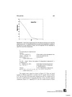
IGURE
6.1A The instantaneous autocorrelation function of a two-cycle cosine
wave plotted as a three-dimensional plot.
F
IGURE
6.1B The instantaneous autocorrelation function of a two-cycle cosine
wave plotted as a contour plot. The sinusoidal peaks are apparent along both
axes as well as along the diagonals.
TLFeBOOK
152 Chapter 6
of the instantaneous autocorrelation function, but only along the τ (i.e., lag)
dimension. The result is a function of both frequency and time. When the one-
dimensional power spectrum was computed using the autocorrelation function,
it was common to filter the autocorrelation function before taking the Fourier
transform to improve features of the resulting power spectrum. While no such
filtering is done in constructing the Wigner-Ville distribution, all of the other
approaches apply a filter (in this case a two-dimensional filter) to the instanta-
neous autocorrelation function before taking the Fourier transform. In fact, the
primary difference between many of the distributions in Cohen’s class is simply
the type of filter that is used.
The formal equation for determining a time–frequency distribution from
Cohen’s class of distributions is rather formidable, but can be simplified in
practice. Specifically, the general equation is:

ρ(t,f) = ∫∫∫g(v,τ)e
j2πv(u −τ)
x(u +
1
2
τ)x*(u −
1
2
τ)e
−j2πfr
dv du dτ (8)
where g(v,τ) provides the two-dimensional filtering of the instantaneous auto-
correlation and is also know as a kernel. It is this filter-like function that differ-
entiates between the various distributions in Cohen’s class. Note that the rest
of the integrand is the Fourier transform of the instantaneous autocorrelation
function.
There are several ways to simplify Eq. (8) for a specific kernel. For the
Wigner-Ville distribution, there is no filtering, and the kernel is simply 1 (i.e.,
g(v,τ) = 1) and the general equation of Eq. (8), after integration by dv, reduces
to Eq. (9), presented in both continuous and discrete form.
W(t,f) =
∫
∞
−∞
e
−j2 πf τ
x(t −
τ
2
)x(t −

τ
2
)dτ (9a)
W(n,m) = 2
∑
∞
k=−∞
e
−2πnm/N
x(n + k)x*(n − k)(9b)
W(n,m) =
∑
∞
m=−∞
e
−2πnm/N
R
x
(n,k) = FFT
k
[R
x
(n,k)] (9c)
Note that t = nT
s
,andf = m/(NT
s
)
The Wigner-Ville has several advantages over the STFT, but also has a
number of shortcomings. It greatest strength is that produces “a remarkably

good picture of the time-frequency structure” (Cohen, 1992). It also has favor-
able marginals and conditional moments. The marginals relate the summation
over time or frequency to the signal energy at that time or frequency. For exam-
ple, if we sum the Wigner-Ville distribution over frequency at a fixed time, we
get a value equal to the energy at that point in time. Alternatively, if we fix
TLFeBOOK
Time–Frequency Analysis 153
frequency and sum over time, the value is equal to the energy at that frequency.
The conditional moment of the Wigner-Ville distribution also has significance:
f
inst
=
1
p(t)
∫
∞
−∞
fρ(f,t)df (10)
where p(t) is the marginal in time.
This conditional moment is equal to the so-called instantaneous fre-
quency. The instantaneous frequency is usually interpreted as the average of the
frequencies at a given point in time. In other words, treating the Wigner-Ville
distribution as an actual probability density (it is not) and calculating the mean
of frequency provides a term that is logically interpreted as the mean of the
frequencies present at any given time.
The Wigner-Ville distribution has a number of other properties that may
be of value in certain applications. It is possible to recover the original signal,
except for a constant, from the distribution, and the transformation is invariant
to shifts in time and frequency. For example, shifting the signal in time by a
delay of T seconds would produce the same distribution except shifted by T on

the time axis. The same could be said of a frequency shift (although biological
processes that produce shifts in frequency are not as common as those that
produce time shifts). These characteristics are also true of the STFT and some
of the other distributions described below. A property of the Wigner-Ville distri-
bution not shared by the STFT is finite support in time and frequency. Finite
support in time means that the distribution is zero before the signal starts and
after it ends, while finite support in frequency means the distribution does not
contain frequencies beyond the range of the input signal. The Wigner-Ville does
contain nonexistent energies due to the cross products as mentioned above and
observed in Figure 6.1, but these are contained within the time and frequency
boundaries of the original signal. Due to these cross products, the Wigner-Ville
distribution is not necessarily zero whenev er the signal is zero, a proper ty Cohen
called strong finite support. Ob vious ly, since the STFT does not have finite sup-
port it does not have strong finite support. A few of the other distributions do
have strong finite support. Examples of the desirable attributes of the Wigner-Ville
will be explored in the MATLAB Implementation section, and in the problems.
The Wigner-Ville distribution has a number of shortcomings. Most serious
of these is the production of cross products: the demonstration of energies at
time–frequency values where they do not exist. These phantom energies have
been the prime motivator for the development of other distributions that apply
various filters to the instantaneous autocorrelation function to mitigate the dam-
age done by the cross products. In addition, the Wigner-Ville distribution can
have negative regions that have no meaning. The Wigner-Ville distribution also
has poor noise properties. Essentially the noise is distributed across all time and
TLFeBOOK
154 Chapter 6
frequency including cross products of the noise, although in some cases, the
cross products and noise influences can be reduced by using a window. In
such cases, the desired window function is applied to the lag dimension of the
instantaneous autocorrelation function (Eq. (7)) similar to the way it was applied

to the time function in Chapter 3. As in Fourier transform analysis, windowing
will reduce frequency resolution, and, in practice, a compromise is sought be-
tween a reduction of cross products and loss of frequency resolution. Noise
properties and the other weaknesses of the Wigner-Ville distribution along with
the influences of windowing are explored in the implementation and problem
sections.
The Choi-Williams and Other Distributions
The existence of cross products in the Wigner-Ville transformation has motived
the development of other distributions. These other distributions are also defined
by Eq. (8); however, now the kernel, g(v,τ), is no longer 1. The general equation
(Eq. (8)) can be simplified two different ways: for any given kernel, the integra-
tion with respect to the variable v can be performed in advance since the rest of
the transform (i.e., the signal portion) is not a function of v; or use can be made
of an intermediate function, called the ambiguity function.
In the first approach, the kernel is multiplied by the exponential in Eq. (9)
to give a new function, G(u,τ):
G(u,τ) =
∫
∞
−∞
g(v,τ)e
jπvu
dv (11)
where the new function, G(u,τ) is referred to as the determining function
(Boashash and Reilly, 1992). Then Eq. (9) reduces to:
ρ(t,f) =∫∫G(u − t,τ)x(u +
1
2
τ)x*(u −
1

2
τ)e
−2πf τ
dudτ (12)
Note that the second set of terms under the double integral is just the
instantaneous autocorrelation function given in Eq. (7). In terms of the determin-
ing function and the instantaneous autocorrelation function, the discrete form of
Eq. (12) becomes:
ρ(t,f) =
∑
M
τ=0
R
x
(t,τ)G(t,τ)e
−j2 πf τ
(13)
where t = u/f
s
. This is the approach that is used in the section on MATLAB
implementation below. Alternatively, one can define a new function as the in-
verse Fourier transform of the instantaneous autocorrelation function:
A
x
(θ,τ)
∆
=
IFT
t
[x(t +τ/2)x*(t −τ/2)] = IFT

t
[R
x
(t,τ)] (14)
TLFeBOOK
Time–Frequency Analysis 155
where the new function, A
x
(θ,τ), is termed the ambiguity function. In this case,
the convolution operation in Eq. (13) becomes multiplication, and the desired
distribution is just the double Fourier transform of the product of the ambiguity
function times the instantaneous autocorrelation function:
ρ(t,f) = FFT
t
{FFT
f
[A
x
(θ,τ)R
x
(t,τ)]} (15)
One popular distribution is the Choi-Williams, which is also referred to as
an exponential distribution (ED) since it has an exponential-type kernel. Specifi-
cally, the kernel and determining function of the Choi-Williams distribution
are:
g(v,τ) = e
−v
2
τ
2

/σ
(16)
After integrating the equation above as in Eq. (11), G(t,τ) becomes:
G(t,τ) =
√
σ/π
2τ
e
−σt
2
/4τ
2
(17)
The Choi-Williams distribution can also be used in a modified form that
incorporates a window function and in this form is considered one of a class of
reduced interference distributions (RID) (Williams, 1992). In addition to having
reduced cross products, the Choi-Williams distribution also has better noise
characteristics than the Wigner-Ville. These two distributions will be compared
with other popular distributions in the section on implementation.
Analytic Signal
All of the transformations in Cohen’s class of distributions produce better results
when applied to a modified version of the waveform termed the Analytic signal,
a complex version of the real signal. While the real signal can be used, the
analytic signal has several advantages. The most important advantage is due to
the fact that the analytic signal does not contain negative frequencies, so its use
will reduce the number of cross products. If the real signal is used, then both
the positive and negative spectral terms produce cross products. Another benefit
is that if the analytic signal is used the sampling rate can be reduced. This is
because the instantaneous autocorrelation function is calculated using evenly
spaced values, so it is, in fact, undersampled by a factor of 2 (compare the

discrete and continuous versions of Eq. (9)). Thus, if the analytic function is
not used, the data must be sampled at twice the normal minimum; i.e., twice
the Nyquist frequency or four times f
MAX
.* Finally, if the instantaneous frequency
*If the waveform has already been sampled, the number of data points should be doubled with
intervening points added using interpolation.
TLFeBOOK
156 Chapter 6
is desired, it can be determined from the first moment (i.e., mean) of the distri-
bution only if the analytic signal is used.
Several approaches can be used to construct the analytic signal. Essen-
tially one takes the real signal and adds an imaginary component. One method
for establishing the imaginary component is to argue that the negative frequen-
cies that are generated from the Fourier transform are not physical and, hence,
should be eliminated. (Negative frequencies are equivalent to the redundant fre-
quencies above f
s
/2. Following this logic, the Fourier transform of the real signal
is taken, the negative frequencies are set to zero, or equivalently, the redundant
frequencies above f
s
/2, and the (now complex) signal is reconstructed using the
inverse Fourier transform. This approach also multiplies the positive frequen-
cies, those below f
s
/2, by 2 to keep the overall energy the same. This results in
a new signal that has a real part identical to the real signal and an imaginary
part that is the Hilbert Transform of the real signal (Cohen, 1989). This is the
approach used by the MATLAB routine

hilbert
and the routine
hilber
on
the disk, and the approach used in the examples below.
Another method is to perform the Hilbert transform directly using the
Hilbert transform filter to produce the complex component:
z(n) = x(n) + j H[x(n)] (18)
where H denotes the Hilbert transform, which can be implemented as an FIR
filter (Chapter 4) with coefficients of:
h(n) =
ͭ
2 sin
2
(πn/2)
πn
for n ≠ 0
0forn = 0
(19)
Although the Hilbert transform filter should have an infinite impulse re-
sponse length (i.e., an infinite number of coefficients), in practice an FIR filter
length of approximately 79 samples has been shown to provide an adequate
approximation (Bobashash and Black, 1987).
MATLAB IMPLEMENTATION
The Short-Term Fourier Transform
The implementation of the time–frequency al gorit hms described above is s traig ht-
forward and is illustrated in the examples below. The spectrogram can be gener-
ated using the standard
fft
function described in Chapter 3, or using a special

function of the Signal Processing Toolbox,
specgram
. The arguments for
spec-
gram
(given on the next page) are similar to those use for
pwelch
described in
Chapter 3, although the order is different.
TLFeBOOK
Time–Frequency Analysis 157
[B,f,t] = specgram(x,nfft,fs,window,noverlap)
where the output,
B
, is a complex matrix containing the magnitude and phase of
the STFT time–frequency spectrum with the rows encoding the time axis and
the columns representing the frequency axis. The optional output arguments,
f
and
t
, are time and frequency vectors that can be helpful in plotting. The input
arguments include the data vector,
x
, and the size of the Fourier transform win-
dow,
nfft
. Three optional input arguments include the sampling frequency,
fs
,
used to calculate the plotting vectors, the window function desired, and the

number of overlapping points between the windows. The window function is
specified as in
pwelch
: if a scalar is given, then a Hanning window of that
length is used.
The output of all MATLAB-based time–frequency methods is a function
of two variables, time and frequency, and requires either a three-dimensional
plot or a two-dimensional contour plot. Both plotting approaches are available
through MATLAB standard graphics and are illustrated in the example below.
Example 6.1 Construct a time series consisting of two sequential sinu-
soids of 10 and 40 Hz, each active for 0.5 sec (see Figure 6.2). The sinusoids
should be preceded and followed by 0.5 sec of no signal (i.e., zeros). Determine
the magnitude of the STFT and plot as both a three-dimensional grid plot and
as a contour plot. Do not use the Signal Processing Toolbox routine, but develop
code for the STFT. Use a Hanning window to isolate data segments.
Example 6.1 uses a function similar to MATLAB’s
specgram
, except that
the window is fixed (Hanning) and all of the input arguments must be specified.
This function,
spectog
, has arguments similar to those in
specgram
. The code
for this routine is given below the main program.
F
IGURE
6.2 Waveform used in Example 6.1 consisting of two sequential sinu-
soids of 10 and 40 Hz. Only a portion of the 0.5 sec endpoints are shown.
TLFeBOOK

158 Chapter 6
% Example 6.1 and Figures 6.2, 6.3, and 6.4
% Example of the use of the spectrogram
% Uses function spectog given below
%
clear all; close all;
% Set up constants
fs = 500; % Sample frequency in Hz
N = 1024; % Signal length
f1 = 10; % First frequency in Hz
f2 = 40; % Second frequency in Hz
nfft = 64; % Window size
noverlap = 32; % Number of overlapping points (50%)
%
% Construct a step change in frequency
tn = (1:N/4)/fs; % Time vector used to create sinusoids
x = [zeros(N/4,1); sin(2*pi*f1*tn)’; sin(2*pi*f2*tn)’
zeros(N/4,1)];
t = (1:N)/fs; % Time vector used to plot
plot(t,x,’k’);
labels
% Could use the routine specgram from the MATLAB Signal Processing
% Toolbox: [B,f,t] = specgram(x,nfft,fs,window,noverlap),
% but in this example, use the “spectog” function shown below.
F
IGURE
6.3 Contour plot of the STFT of two sequential sinusoids. Note the broad
time and frequency range produced by this time–frequency approach. The ap-
pearance of energy at times and frequencies where no energy exists in the origi-
nal signal is evident.

TLFeBOOK
Time–Frequency Analysis 159
F
IGURE
6.4 Time–frequency magnitude plot of the waveform in Figure 6.3 using
the three-dimensional grid technique.
%
[B,f,t] = spectog(x,nfft,fs,noverlap);
B = abs(B); % Get spectrum magnitude
figure;
mesh(t,f,B); % Plot Spectrogram as 3-D mesh
view(160,40); % Change 3-D plot view
axis([0 2 0 100 0 20]); % Example of axis and
xlabel(’Time (sec)’); % labels for 3-D plots
ylabel(’Frequency (Hz)’);
figure
contour(t,f,B); % Plot spectrogram as contour plot
labels and axis
The function
spectog
is coded as:
function [sp,f,t] = spectog(x,nfft,fs,noverlap);
% Function to calculate spectrogram
TLFeBOOK
160 Chapter 6
% Output arguments
% sp spectrogram
% t time vector for plotting
% f frequency vector for plotting
% Input arguments

% x data
% nfft window size
% fs sample frequency
% noverlap number of overlapping points in adjacent segments
% Uses Hanning window
%
[N xcol] = size(x);
if N < xcol
x = x’; % Insure that the input is a row
N = xcol; % vector (if not already)
end
incr = nfft—noverlap; % Calculate window increment
hwin = fix(nfft/2); % Half window size
f = (1:hwin)*(fs/nfft); % Calculate frequency vector
% Zero pad data array to handle edge effects
x_mod = [zeros(hwin,1); x; zeros(hwin,1)];
%
j = 1; % Used to index time vector
% Calculate spectra for each window position
% Apply Hanning window
for i = 1:incr:N
data = x_mod(i:i؉nfft-1) .* hanning(nfft);
ft = abs(fft(data)); % Magnitude data
sp(:,j) = ft(1:hwin); % Limit spectrum to meaningful
% points
t(j) = i/fs; % Calculate time vector
j = j ؉ 1; % Increment index
end
Figures 6.3 and 6.4 show that the STFT produces a time–frequency plot
with the step change in frequency at approximately the correct time, although

neither the step change nor the frequencies are very precisely defined. The lack
of finite support in either time or frequency is evidenced by the appearance of
energy slightly before 0.5 sec and slightly after 1.5 sec, and energies at frequen-
cies other than 10 and 40 Hz. In this example, the time resolution is better than
the frequency resolution. By changing the time window, the compromise be-
tween time and frequency resolution could be altered. Exploration of this trade-
off is given as a problem at the end of this chapter.
A popular signal used to explore the behavior of time–frequency methods
is a sinusoid that increases in frequency over time. This signal is called a chirp
TLFeBOOK
Time–Frequency Analysis 161
signal because of the sound it makes if treated as an audio signal. A sample of
such a signal is shown in Figure 6.5. This signal can be generated by multiplying
the argument of a sine function by a linearly increasing term, as shown in Exam-
ple 6.2 below. Alternatively, the Signal Processing Toolbox contains a special
function to generate a chip that provides some extra features such as logarithmic
or quadratic changes in frequency. The MATLAB
chirp
routine is used in a
latter example. The output of the STFT to a chirp signal is demonstrated in
Figure 6.6.
Example 6.2 Generate a linearly increasing sine wave that varies be-
tween 10 and 200 Hz over a 1sec period. Analyze this chirp signal using the
STFT program used in Example 6.1. Plot the resulting spectrogram as both a 3-
D grid and as a contour plot. Assume a sample frequency of 500 Hz.
% Example 6.2 and Figure 6.6
% Example to generate a sine wave with a linear change in frequency
% Evaluate the time–frequency characteristic using the STFT
% Sine wave should vary between 10 and 200 Hz over a 1.0 sec period
% Assume a sample rate of 500 Hz

%
clear all; close all;
% Constants
N = 512; % Number of points
F
IGURE
6.5 Segment of a chirp signal, a signal that contains a single sinusoid
that changes frequency over time. In this case, signal frequency increases linearly
with time.
TLFeBOOK
162 Chapter 6
F
IGURE
6.6 The STFT of a chirp signal, a signal linearly increasing in frequency
from 10 to 200 Hz, shown as both a 3-D grid and a contour plot.
fs = 500; % Sample freq;
f1 = 10; % Minimum frequency
f2 = 200; % Maximum frequency
nfft = 32; % Window size
t = (1:N)/fs; % Generate a time
% vector for chirp
% Generate chirp signal (use a linear change in freq)
fc = ((1:N)*((f2-f1)/N)) ؉ f1;
x = sin(pi*t.*fc);
%
% Compute spectrogram using the Hanning window and 50% overlap
[B,f,t] = spectog(x,nfft,fs,nfft/2); % Code shown above
%
subplot(1,2,1); % Plot 3-D and contour
% side-by-side

mesh(t,f,abs(B)); % 3-D plot
labels, axis, and title
subplot(1,2,2);
contour(t,f,abs(B)); % Contour plot
labels, axis, and title
The Wigner-Ville Distribution
The Wigner-Ville distribution will provide a much more definitive picture of
the time–frequency characteristics, but will also produce cross products: time–
TLFeBOOK
Time–Frequency Analysis 163
frequency energy that is not in the original signal, although it does fall within
the time and frequency boundaries of the signal. Example 6.3 demonstrates these
properties on a signal that changes frequency abruptly, the same signal used in
Example 6.1with the STFT. This will allow a direct comparison of the two
methods.
Example 6.3 Appl y the Wigner-Ville distribut ion to the si gna l of Exam -
ple 6.1. Use the analytic signal and provide plots simil ar to those of Example 6.1.
% Example 6.3 and Figures 6.7 and 6.8
% Example of the use of the Wigner-Ville distribution
% Applies the Wigner-Ville to data similar to that of Example
% 6.1, except that the data has been shortened from 1024 to 512
% to improve run time.
%
clear all; close all;
% Set up constants (same as Example 6–1)
fs = 500; % Sample frequency
N = 512; % Signal length
f1 = 10; % First frequency in Hz
f2 = 40; % Second frequency in Hz
F

IGURE
6.7 Wigner-Ville distribution for the two sequential sinusoids shown in
Figure 6.3. Note that while both the frequency ranges are better defined than
in Figure 6.2 produced by the STFT, there are large cross products generated in
the region between the two actual signals (central peak). In addition, the distribu-
tions are sloped inward along the time axis so that onset time is not as precisely
defined as the frequency range.
TLFeBOOK
164 Chapter 6
F
IGURE
6.8 Contour plot of the Wigner-Ville distribution of two sequential sinu-
soids. The large cross products are clearly seen in the region between the actual
signal energy. Again, the slope of the distributions in the time domain make it
difficult to identify onset times.
%
% Construct a step change in frequency as in Ex. 6–1
tn = (1:N/4)/fs;
x = [zeros(N/4,1); sin(2*pi*f1*tn)’; sin(2*pi*f2*tn)’;
zeros(N/4,1)];
%
% Wigner-Ville analysis
x = hilbert(x); % Construct analytic function
[WD,f,t] = wvd(x,fs); % Wigner-Ville transformation
WD = abs(WD); % Take magnitude
mesh(t,f,WD); % Plot distribution
view(100,40); % Use different view
Labels and axis
figure
contour(t,f,WD); % Plot as contour plot

Labels and axis
The function
wwd
computes the Wigner-Ville distribution.
function [WD,f,t] = wvd(x,fs)
% Function to compute Wigner-Ville time–frequency distribution
% Outputs
% WD Wigner-Ville distribution
% f Frequency vector for plotting
% t Time vector for plotting
TLFeBOOK
Time–Frequency Analysis 165
% Inputs
% x Complex signal
% fs Sample frequency
%
[N, xcol] = size(x);
if N < xcol % Make signal a column vector if necessary
x = x!; % Standard (non-complex) transpose
N = xcol;
end
WD = zeros(N,N); % Initialize output
t = (1:N)/fs; % Calculate time and frequency vectors
f = (1:N)*fs/(2*N);
%
%
%Compute instantaneous autocorrelation: Eq. (7)
for ti = 1:N % Increment over time
taumax = min([ti-1,N-ti,round(N/2)-1]);
tau = -taumax:taumax;

% Autocorrelation: tau is in columns and time is in rows
WD(tau-tau(1)؉1,ti) = x(ti؉tau) .* conj(x(ti-tau));
end
%
WD = fft(WD);
The last section of code is used to compute the instantaneous autocorrela-
tion function and its Fourier transform as in Eq. (9c). The
for
loop is used to
construct an array,
WD
, containing the instantaneous autocorrelation where each
column contains the correlations at various lags for a given time,
ti
. Each
column is computed over a range of lags, ±
taumax
. The first statement in the
loop restricts the range of
taumax
to be within signal array: it uses all the data
that is symmetrically available on either side of the time variable,
ti
. Note that
the phase of the lag signal placed in array
WD
varies by column (i.e., time).
Normally this will not matter since the Fourier transform will be taken over
each set of lags (i.e., each column) and only the magnitude will be used. How-
ever, the phase was properly adjusted before plotting the instantaneous autocor-

relation in Figure 6.1. After the instantaneous autocorrelation is constructed, the
Fourier transform is taken over each set of lags. Note that if an array is presented
to the MATLAB
fft
routine, it calculates the Fourier transform for each col-
umn; hence, the Fourier transform is computed for each value in time producing
a two-dimensional function of time and frequency.
The Wigner-Ville is particularly effective at detecting single sinusoids that
change in frequency with time, such as the chirp signal shown in Figure 6.5 and
used in Example 6.2. For such signals, the Wigner-Ville distribution produces
very few cross products, as shown in Example 6.4.
TLFeBOOK
166 Chapter 6
Example 6.4 Apply the Wigner-Ville distribution to a chirp signal the
ranges linearly between 20 and 200 Hz over a 1 second time period. In this
example, use the MATLAB
chirp
routine.
% Example 6.4 and Figure 6.9
% Example of the use of the Wigner-Ville distribution applied to
% a chirp
% Generates the chirp signal using the MATLAB chirp routine
%
clear all; close all;
% Set up constants % Same as Example 6.2
fs = 500; % Sample frequency
N = 512; % Signal length
f1 = 20; % Starting frequency in Hz
f2 = 200; % Frequency after 1 second (end)
%inHz

%
% Construct “chirp” signal
tn = (1:N)/fs;
F
IGURE
6.9 Wigner-Ville of a chirp signal in which a single sine wave increases
linearly with time. While both the time and frequency of the signal are well-
defined, the amplitude, which should be constant, varies considerably.
TLFeBOOK
Time–Frequency Analysis 167
x = chirp(tn,f1,1,f2)’; % MATLAB routine
%
% Wigner-Ville analysis
x = hilbert(x); % Get analytic function
[WD,f,t] = wvd(x,fs); % Wigner-Ville—see code above
WD = abs(WD); % Take magnitude
mesh(t,f,WD); % Plot in 3-D
3D labels, axis, view
If the analytic signal is not used, then the Wigner-Ville generates consider-
ably more cross products. A demonstration of the advantages of using the ana-
lytic signal is given in Problem 2 at the end of the chapter.
Choi-Williams and Other Distributions
To implement other distributions in Cohen’s class, we will use the approach
defined by Eq. (13). Following Eq. (13), the desired distribution can be obtained
by convolving the related determining function (Eq. (17)) with the instantaneous
autocorrelation function (R
x
(t,τ); Eq. (7)) then taking the Fourier transform with
respect to τ. As mentioned, this is simply a two-dimensional filtering of the
instantaneous autocorrelation function by the appropriate filter (i.e., the deter-

mining function), in this case an exponential filter. Calculation of the instanta-
neous autocorrelation function has already been done as part of the Wigner-Ville
calculation. To facilitate evaluation of the other distributions, we first extract the
code for the instantaneous autocorrelation from the Wigner-Ville function,
wvd
in Example 6.3, and make it a separate function that can be used to determine
the various distributions. This function has been termed
int_autocorr
, and
takes the data as input and produces the instantaneous autocorrelation function
as the output. These routines are available on the CD.
function Rx = int_autocorr(x)
% Function to compute the instantenous autocorrelation
% Output
% Rx instantaneous autocorrelation
% Input
% x signal
%
[N, xcol] = size(x);
Rx = zeros(N,N); % Initialize output
%
% Compute instantaneous autocorrelation
for ti = 1:N % Increment over time
taumax = min([ti-1,N-ti,round(N/2)-1]);
tau = -taumax:taumax;
TLFeBOOK
168 Chapter 6
Rx(tau-tau(1)؉1,ti) = x(ti؉tau) .* conj(x(ti-tau));
end
The various members of Cohen’s class of distributions can now be imple-

mented by a general routine that starts with the instantaneous autocorrelation
function, evaluates the appropriate determining funct ion, filters the instantaneous
autocorrelation function by the determining function using convolution, then
takes the Fourier transform of the result. The routine described below,
cohen
,
takes the data, sample interval, and an argument that specifies the type of distri-
bution desired and produces the distribution as an output along with time and
frequency vectors useful for plotting. The routine is set up to evaluate four
different distributions: Choi-Williams, Born-Jorden-Cohen, Rihaczek-Marge-
nau, with the Wigner-Ville distribution as the default. The function also plots
the selected determining function.
function [CD,f,t] = cohen(x,fs,type)
% Function to compute several of Cohen’s class of time–frequencey
% distributions
%
% Outputs
% CD Desired distribution
% f Frequency vector for plotting
% t Time vector for plotting
%Inputs
% x Complex signal
% fs Sample frequency
% type of distribution. Valid arguements are:
% ’choi’ (Choi-Williams), ’BJC’ (Born-Jorden-Cohen);
% and ’R_M’ (Rihaczek-Margenau) Default is Wigner-Ville
%
% Assign constants and check input
sigma = 1; % Choi-Williams constant
L = 30; % Size of determining function

%
[N, xcol] = size(x);
if N < xcol % Make signal a column vector if
x = x’; % necessary
N = xcol;
end
t = (1:N)/fs; % Calculate time and frequency
f = (1:N) *(fs/(2*N)); % vectors for plotting
%
% Compute instantaneous autocorrelation: Eq. (7)
TLFeBOOK
Time–Frequency Analysis 169
CD = int_autocorr(x);
if type(1) == ’c’ % Get appropriate determining
% function
G = choi(sigma,L); % Choi-Williams
elseif type(1) == ’B’
G = BJC(L); % Born-Jorden-Cohen
elseif type(1) == ’R’
G = R_M(L); % Rihaczek-Margenau
else
G = zeros(N,N); % Default Wigner-Ville
G(N/2,N/2) = 1;
end
%
figure
mesh(1:L-1,1:L-1,G); % Plot determining function
xlabel(’N’); ylabel(’N’); % and label axis
zlabel(’G(,N,N)’);
%

% Convolve determining function with instantaneous
% autocorrelation
CD = conv2(CD,G); % 2-D convolution
CD = CD(1:N,1:N); % Truncate extra points produced
% by convolution
%
% Take FFT again, FFT taken with respect to columns
CD = flipud(fft(CD)); % Output distribution
The code to produce the Choi-Williams determining function is a straight-
forward implementation of G(t,τ) in Eq. (17) as shown below. The function is
generated for only the first quadrant, then duplicated in the other quadrants. The
function itself is plotted in Figure 6.10. The code for other determining functions
follows the same general structure and can be found in the software accompany-
ing this text.
function G = choi(sigma,N)
% Function to calculate the Choi-Williams distribution function
% (Eq. (17)
G(1,1) = 1; % Compute one quadrant then expand
for j = 2:N/2
wt = 0;
for i = 1:N/2
G(i,j) = exp(-(sigma*(i-1)v2)/(4*(j-1)v2));
wt = wt ؉ 2*G(i,j);
end
TLFeBOOK
170 Chapter 6
F
IGURE
6.10 The Choi-Williams determining function generated by the code below.
wt = wt—G(1,j); % Normalize array so that

% G(n,j) = 1
for i = 1:N/2
G(i,j) = G(i,j)/wt;
end
end
%
% Expand to 4 quadrants
G = [ fliplr(G(:,2:end)) G]; % Add 2nd quadrant
G = [flipud(G(2:end,:)); G]; % Add 3rd and 4th quadrants
To complete the package, Example 6.5 provides code that generates the
data (either two sequential sinusoids or a chirp signal), asks for the desired
distributions, evaluates the distribution using the function
cohen
, then plots the
result. Note that the code for implementing Cohen’s class of distributions is
written for educational purposes only. It is not very efficient, since many of the
operations involve multiplication by zero (for example, see Figure 6.10 and
Figure 6.11), and these operations should be eliminated in more efficient code.
TLFeBOOK
Time–Frequency Analysis 171
F
IGURE
6.11 The determining function of the Rihaczek-Margenau distribution.
Example 6.5 Compare the Choi-Williams and Rihaczek-Margenau dis-
tributions for both a double sinusoid and chirp stimulus. Plot the Rihaczek-
Margenau determining function* and the results using 3-D type plots.
% Example 6.5 and various figures
% Example of the use of Cohen’s class distributions applied to
% both sequential sinusoids and a chirp signal
%

clear all; close all;
global G;
% Set up constants. (Same as in previous examples)
fs = 500; % Sample frequency
N = 256; % Signal length
f1 = 20; % First frequency in Hz
f2 = 100; % Second frequency in Hz
%
% Construct a step change in frequency
signal_type = input (’Signal type (1 = sines; 2 = chirp):’);
if signal_type == 1
tn = (1:N/4)/fs;
x = [zeros(N/4,1); sin(2*pi*f1*tn)’; sin(2*pi*f2*tn)’;
*Note the code for the Rihaczek-Margenau determining function and several other determining
functions can be found on disk with the software associated with this chapter.
TLFeBOOK
172 Chapter 6
zeros(N/4,1)];
else
tn = (1:N)/fs;
x = chirp(tn,f1,.5,f2)’;
end
%
%
% Get desired distribution
type = input(’Enter type (choi,BJC,R_M,WV):’,’s’);
%
x = hilbert(x); % Get analytic function
[CD,f,t] = cohen(x,fs,type); % Cohen’s class of
% transformations

CD = abs(CD); % Take magnitude
% % Plot distribution in
figure; % 3-D
mesh(t,f,CD);
view([85,40]); % Change view for better
% display
3D labels and scaling
heading = [type ’ Distribution’]; % Construct appropriate
eval([’title(’,’heading’, ’);’]); % title and add to plot
%
%
figure;
contour(t,f,CD); % Plot distribution as a
contour plot
xlabel(’Time (sec)’);
ylabel(’Frequency (Hz)’);
eval([’title(’,’heading’, ’);’]);
This program was used to generate Figures 6.11–6.15.
In this chapter we have explored only a few of the many possible time–
frequency distributions, and, necessarily, covered only the very basics of this
extensive subject. Two of the more important topics that were not covered here
are the estimation of instantaneous frequency from the time–frequency distribu-
tion, and the effect of noise on these distributions. The latter is covered briefly
in the problem set below.
PROBLEMS
1. Construct a chirp signal similar to that used in Example 6.2. Evaluate the
analysis characteristics of the STFT using different window filters and sizes.
Specifically, use window sizes of 128, 64, and 32 points. Repeat this analysis
TLFeBOOK
F

IGURE
6.12 Choi-Williams distribution for the two sequential sinusoids shown
in Figure 6.3. Comparing this distribution with the Wigner-Ville distribution of the
same stimulus, Figure 6.7, note the decreased cross product terms.
F
IGURE
6.13 The Rihaczek-Margenau distribution for the sequential sinusoid
signal. Note the very low value of cross products.
173
TLFeBOOK