Biosignal and Biomedical Image Processing MATLAB-Based Applications Muya phần 10 potx

Image Segmentation 359
F
IGURE
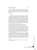
12.13 Isolated segments produced by thresholding the lowpass filtered
image in Figure 12.12. The rightmost segment was found by applying logical op-
erations to the other two images.
%
% Define filters and functions: I-D range function
range = inline(‘max(x)—min(x)’);
h_lp = fspecial (‘gaussian’, 20, 4);
%
% Directional nonlinear filter
I_nl = nlfilter(I, [9 1], range);
I_h = imfilter(I_nl*2, h_lp); % Average (lowpass filter)
%
subplot(2,2,1); imshow % Display image and histogram
(I_nl*2); % before lowpass filtering
title(‘Modified Image’); % and after lowpass filtering
subplot(2,2,2); imhist(I_nl);
title(‘Histogram’);
subplot(2,2,3); imshow(I_h*2); % Display modified image
title(‘Modified Image’);
subplot(2,2,4); imhist(I_h);
title(‘Histogram’);
%
figure;
BW1 = im2bw(I_h,.08); % Threshold to isolate segments
BW2 = ϳim2bw(I_h,.29);
BW3 = ϳ(BW1 & BW2); % Find third image from other
% two
subplot(1,3,1); imshow(BW1); % Display segments

subplot(1,3,2); imshow(BW2);
subplot(1,3,3); imshow(BW3);
TLFeBOOK
360 Chapter 12
The image produced by the horizontal range operator with, and without,
lowpass filtering is shown in Figure 12.12. Note the improvement in separation
produced by the lowpass filtering as indicated by a better defined histogram.
The thresholded images are shown in Figure 12.13. As in Example 12.2, the
separation is not perfect, but is quite good considering the challenges posed by
the original image.
Multi-Thresholding
The results of several different segmentation approaches can be combined either
by adding the images together or, more commonly, by first thresholding the
images into separate binary images and then combining them using logical oper-
ations. Either the AND or OR operator would be used depending on the charac-
teristics of each segmentation procedure. If each procedure identified all of the
segments, but also included non-desired areas, the AND operator could be used
to reduce artifacts. An example of the use of the AND operation was found
in Example 12.3 where one segment was found using the inverse of a logical
AND of the other two segments. Alternatively, if each procedure identified
some portion of the segment(s), then the OR operator could be used to com-
bine the various portions. This approach is illustrated in Example 12.4 where
first two, then three, thresholded images are combined to improve segment iden-
tification. The structure of interest is a cell which is shown on a gray back-
ground. Threshold levels above and below the gray background are combined
(after one is inverted) to provide improved isolation. Including a third binary
image obtained by thresholding a texture image further improves the identifica-
tion.
Example 12.4 Isolate the cell structures from the image of a cell shown
in Figure 12.14.

Solution Since the cell is projected against a gray background it is possi-
ble to isolate some portions of the cell by thresholding above and below the
background level. After inversion of the lower threshold image (the one that is
below the background level), the images are combined using a logical OR. Since
the cell also shows some textural features, a texture image is constructed by
taking the regional standard deviation (Figure 12.14). After thresholding, this
texture-based image is also combined with the other two images.
% Example 12.4 and Figures 12.14 and 12.15
% Analysis of the image of a cell using texture and intensity
% information then combining the resultant binary images
% with a logical OR operation.
clear all; close all;
I = imread(‘cell.tif’); % Load “orientation” texture
TLFeBOOK
Image Segmentation 361
F
IGURE
12.14 Image of cells (left) on a gray background. The textural image
(right) was created based on local variance (standard deviation) and shows
somewhat more definition. (Cancer cell from rat prostate, courtesy of Alan W.
Partin, M.D., Ph.D., Johns Hopkins University School of Medicine.)
I = im2double(I); % Convert to double
%
h = fspecial(‘gaussian’, 20, 2); % Gaussian lowpass filter
%
subplot(1,2,1); imshow(I); % Display original image
title(‘Original Image’);
I_std = (nlfilter(I,[3 3], % Texture operation
’std2’))*6;
I_lp = imfilter(I_std, h); % Average (lowpass filter)

%
subplot(1,2,2); imshow(I_lp*2); % Display texture image
title(‘Filtered image’);
%
figure;
BW_th = im2bw(I,.5); % Threshold image
BW_thc = ϳim2bw(I,.42); % and its complement
BW_std = im2bw(I_std,.2); % Threshold texture image
BW1 = BW_th * BW_thc; % Combine two thresholded
% images
BW2 = BW_std * BW_th * BW_thc; % Combine all three images
subplot(2,2,1); imshow(BW_th); % Display thresholded and
subplot(2,2,2); imshow(BW_thc); % combined images
subplot(2,2,3); imshow(BW1);
TLFeBOOK
362 Chapter 12
F
IGURE
12.15 Isolated portions of the cells shown in Figure 12.14. The upper
images were created by thresholding the intensity. The lower left image is a com-
bination (logical OR) of the upper images and the lower right image adds a
thresholded texture-based image.
The original and texture images are shown in Figure 12.14. Note that the
texture image has been scaled up, first by a factor of six, then by an additional
factor of two, to bring it within a nominal image range. The intensity thresh-
olded images are shown in Figure 12.15 (upper images; the upper right image
has been inverted). These images are combined in the lower left image. The
lower right image shows the combination of both intensity-based images with
the thresholded texture image. This method of combining images can be ex-
tended to any number of different segmentation approaches.

MORPHOLOGICAL OPERATIONS
Morphological operations have to do with processing shapes. In this sense they
are continuity-based techniques, but in some applications they also operate on
TLFeBOOK
Image Segmentation 363
edges, making them useful in edge-based approaches as well. In fact, morpho-
logical operations have many image processing applications in addition to seg-
mentation, and they are well represented and supported in the MATLAB Image
Processing Toolbox.
The two most common morphological operations are dilation and erosion.
In dilation the rich get richer and in erosion the poor get poorer. Specifically,
in dilation, the center or active pixel is set to the maximum of its neighbors,
and in erosion it is set to the minimum of its neighbors. Since these operations
are often performed on binary images, dilation tends to expand edges, borders,
or regions, while erosion tends to decrease or even eliminate small regions.
Obviously, the size and shape of the neighborhood used will have a very strong
influence on the effect produced by either operation.
The two processes can be done in tandem, over the same area. Since both
erosion and dilation are nonlinear operations, they are not invertible transforma-
tions; that is, one followed by the other will not generally result in the original
image. If erosion is followed by dilation, the operation is termed opening.Ifthe
image is binary, this combined operation will tend to remove small objects
without changing the shape and size of larger objects. Basically, the initial ero-
sion tends to reduce all objects, but some of the smaller objects will disappear
altogether. The subsequent dilation will restore those objects that were not elimi-
nated by erosion. If the order is reversed and dilation is performed first followed
by erosion, the combined process is called closing. Closing connects objects
that are close to each other, tends to fill up small holes, and smooths an object’s
outline by filling small gaps. As with the more fundamental operations of dila-
tion and erosion, the size of objects removed by opening or filled by closing

depends on the size and shape of the neighborhood that is selected.
An example of the opening operation is shown in Figure 12.16 including
the erosion and dilation steps. This is applied to the blood cell image after
thresholding, the same image shown in Figure 12.3 (left side). Since we wish
to eliminate black artifacts in the background, we first invert the image as shown
in Figure 12.16. As can be seen in the final, opened image, there is a reduction
in the number of artifacts seen in the background, but there is also now a gap
created in one of the cell walls. The opening operation would be more effective
on the image in which intermediate values were masked out (Figure 12.3, right
side), and this is given as a problem at the end of the chapter.
Figure 12.17 shows an example of closing applied to the same blood cell
image. Again the operation was performed on the inverted image. This operation
tends to fill the gaps in the center of the cells; but it also has filled in gaps
between the cells. A much more effective approach to filling holes is to use the
imfill
routine described in the section on MATLAB implementation.
Other MATLAB morphological routines provide local maxima and min-
ima, and allows for manipulating the image’s maxima and minima, which im-
plement various fill-in effects.
TLFeBOOK
364 Chapter 12
F
IGURE
12.16 Example of the opening operation to remove small artifacts. Note
that the final image has fewer background spots, but now one of the cells has a
gap in the wall.
MATLAB Implementation
The erosion and dilation could be implemented using the nonlinear filter routine
nlfilter
, although this routine limits the shape of the neighborhood to a rect-

angle. The MATLAB routines
imdilate
and
imerode
provide for a variety of
neighborhood shapes and are much faster than
nlfilter
. As mentioned above,
opening consists of erosion followed by dilation and closing is the reverse.
MATLAB also provide routines for implementing these two operations in one
statement.
To specify the neighborhood used by all of these routines, MATLAB uses
a structuring element.* A structuring element can be defined by a binary array,
where the ones represent the neighborhood and the zeros are irrelevant. This
allows for easy specification of neighborhoods that are nonrectangular, indeed
that can have any arbitrary shape. In addition, MATLAB makes a number of
popular shapes directly available, just as the
fspecial
routine makes a number
*Not to be confused with a similar term, structural unit, used in the beginning of this chapter. A
structural unit is the object of interest in the image.
TLFeBOOK
Image Segmentation 365
F
IGURE
12.17 Example of closing to fill gaps. In the closed image, some of the
cells are now filled, but some of the gaps between cells have been erroneously
filled in.
of popular two-dimensional filter functions available. The routine to specify the
structuring element is

strel
and is called as:
structure = strel(shape, NH, arg);
where
shape
is the type of shape desired,
NH
usually specifies the size of the
neighborhood, and
arg
and an argument, frequently optional, that depends on
shape
.If
shape
is
‘arbitrary’
, or simply omitted, then
NH
is an array that
specifies the neighborhood in terms of ones as described above. Prepackaged
shapes include:
‘disk’
a circle of radius
NH
(in pixels)
‘line’
a line of length
NH
and angle
arg

in degrees
‘rectangle’
a rectangle where
NH
is a two element vector specifying rows and col-
umns
‘diamond’
a diamond where
NH
is the distance from the center to each corner
‘square’
a square with linear dimensions
NH
TLFeBOOK
366 Chapter 12
For many of these shapes, the routine
strel
produces a decomposed
structure that runs significantly faster.
Based on the structure, the statements for dilation, erosion, opening, and
closing are:
I1 = imdilate(I, structure);
I1 = imerode(I, structure);
I1 = imopen(I, structuure);
I1 = imclose(I, structure);
where
I1
is the output image,
I
is the input image and

structure
is the neigh-
borhood specification given by
strel
, as described above. In all cases,
struc-
ture
can be replaced by an array specifying the neighborhood as ones, bypass-
ing the
strel
routine. In addition,
imdilate
and
imerode
have optional
arguments that provide packing and unpacking of the binary input or output
images.
Example 12.5 Apply opening and closing to the thresholded blood cell
images of Figure 12–3 in an effort to remove small background artifacts and to
fill holes. Use a circular structure with a diameter of four pixels.
% Example 12.5 and Figures 12.16 and 12.17
% Demonstration of morphological opening to eliminate small
% artifacts and of morphological closing to fill gaps
% These operations will be applied to the thresholded blood cell
% images of Figure 12.3 (left image).
% Uses a circular or disk shaped structure 4 pixels in diameter
%
clear all; close all;
I = imread(‘blood1.tif’); % Get image and threshold
I = im2double(I);

BW = ϳim2bw(I,thresh(I));
%
SE = strel(‘disk’,4); % Define structure: disk of radius
% 4 pixels
BW1= imerode(BW,SE); % Opening operation: erode
BW2 = imdilate(BW1,SE); % image first, then dilate
%
display images
%
BW3= imdilate(BW,SE); % Closing operation, dilate image
BW4 = imerode(BW3,SE); % first then erode
%
display images
TLFeBOOK
Image Segmentation 367
This example produced the images in Figures 12.15 and 12.16.
Example 12.6 Apply an opening operation to remove the dark patches
seen in the thresholded cell image of Figure 12.15.
% Figures 12.6 and 12.18
% Use opening to remove the dark patches in the thresholded cell
% image of Figure 12.15
%
close all; clear all;
%
SE = strel(‘square’,5); % Define closing structure:
% square 5 pixels on a side
load fig12_15; % Get data of Figure 12.15 (BW2)
BW1= ϳimopen(ϳBW2,SE); % Opening operation
Display images
The result of this operation is shown in Figure 12.18. In this case, the

closing operation is able to remove completely the dark patches in the center of
the cell image. A 5-by-5 pixel square structural element was used. The size (and
shape) of the structural element controlled the size of artifact removed, and no
attempt was made to optimize its shape. The size was set here as the minimum
that would still remove all of the dark patches. The opening operation in this
example used the single statement
imopen
. Again, the opening operation oper-
ates on activated (i.e., white pixels), so to remove dark artifacts it is necessary
to invert the image (using the logical NOT operator, ϳ) before performing the
opening operation. The opened image is then inverted again before display.
F
IGURE
12.18 Application of the open operation to remove the dark patches in
the binary cell image in Figure 12.15 (lower right). Using a 5 by 5 square struc-
tural element resulted in eliminating all of the dark patches.
TLFeBOOK
368 Chapter 12
MATLAB morphology routines also allow for manipulation of maxima
and minima in an image. This is useful for identifying objects, and for filling.
Of the many other morphological operations supported by MATLAB, only the
imfill
operation will be described here. This operation begins at a designated
pixel and changes connected background pixels (0’s) to foreground pixels (1’s),
stopping only when a boundary is reached. For grayscale images,
imfill
brings
the intensity levels of the dark areas that are surrounded by lighter areas up to
the same intensity level as surrounding pixels. (In effect,
imfill

removes re-
gional minima that are not connected to the image border.) The initial pixel can
be supplied to the routine or obtained interactively. Connectivity can be defined
as either four connected or eight connected. In four connectivity, only the four
pixels bordering the four edges of the pixel are considered, while in eight con-
nectivity all pixel that touch, including those that touch only at the corners, are
considered connected.
The basic
imfill
statement is:
I_out = imfill(I, [r c], con);
where
I
is the input image,
I_out
is the output image,
[r c]
is a two-element
vector specifying the beginning point, and
con
is an optional argument that is
set to 8 for eight connectivity (four connectivity is the default). (See the help
file to use
imfill
interactively.) A special option of
imfill
is available specifi-
cally for filling holes. If the image is binary, a hole is a set of background pixels
that cannot be reached by filling in the background from the edge of the image.
If the image is an intensity image, a hole is an area of dark pixels surrounded

by lighter pixels. To invoke this option, the argument following the input image
should be
holes
. Figure 12.19 shows the operation performed on the blood cell
image by the statement:
I_out = imfill(I, ‘holes’);
EDGE-BASED SEGMENTATION
Historically, edge-based methods were the first set of tools developed for seg-
mentation. To move from edges to segments, it is necessary to group edges into
chains that correspond to the sides of structural units, i.e., the structural bound-
aries. Approaches vary in how much prior information they use, that is, how
much is used of what is known about the possible shape. False edges and missed
edges are two of the more obvious, and more common, problems associated
with this approach.
The first step in edge-based methods is to identify edges which then be-
come candidates for boundaries. Some of the filters presented in Chapter 11
TLFeBOOK
Image Segmentation 369
F
IGURE
12.19 Hole filling operation produced by
imfill
. Note that neither the
edge cell (at the upper image boundary) or the overlapped cell in the center are
filled since they are not actually holes. (Original image reprinted with permission
from the Image Processing Handbook 2nd edition. Copyright CRC Press, Boca
Raton, Florida.)
perform edge enhancement, including the Sobel, Prewitt, and Log filters. In
addition, the Laplacian, which takes the spatial second derivative, can be used
to find edge candidates. The Canny filter is the most advanced edge detector

supported by MATLAB, but it necessarily produces a binary output while many
of the secondary operations require a graded edge image.
Edge relaxation is one approach used to build chains from individual edge
candidate pixels. This approach takes into account the local neighborhood: weak
edges positioned between strong edges are probably part of the edge, while
strong edges in isolation are likely spurious. The Canny filter incorporates a
type of edge relaxation. Various formal schemes have been devised under this
category. A useful method is described in Sonka (1995) that establishes edges
between pixels (so-called crack edges) based on the pixels located at the end
points of the edge.
Another method for extending edges into chains is termed graph search-
ing. In this approach, the endpoints (which could both be the same point in a
closed boundary) are specified, and the edge is determined based on minimizing
some cost function. Possible pathways between the endpoints are selected from
candidate pixels, those that exceed some threshold. The actual path is selected
based on a minimization of the cost function. The cost function could include
features such as the strength of an edge pixel and total length, curvature, and
proximity of the edge to other candidate borders. This approach allows for a
TLFeBOOK
370 Chapter 12
great deal of flexibility. Finally, dynamic programming can be used which is
also based on minimizing a cost function.
The methods briefly described above use local information to build up the
boundaries of the structural elements. Details of these methods can be found in
Sonka et al. (1995). Model-based edge detection methods can be used to exploit
prior knowledge of the structural unit. For example, if the shape and size of the
image is known, then a simple matching approach based on correlation can be
used (matched filtering). When the general shape is known, but not the size, the
Hough transform can be used. This approach was originally designed for identi-
fying straight lines and curves, but can be expanded to other shapes provided

the shape can be described analytically.
The basic idea behind the Hough transform is to transform the image into
a parameter space that is constructed specifically to describe the desired shape
analytically. Maxima in this parameter space then correspond to the presence of
the desired image in image space. For example, if the desired object is a straight
line (the original application of the Hough transform), one analytic representa-
tion for this shape is y = mx + b,* and such shapes can be completely defined
by a two-dimensional parameter space of m and b parameters. All straight lines
in image space map to points in parameter space (also known as the accumula-
tor array for reasons that will become obvious). Operating on a binary image
of edge pixels, all possible lines through a given pixel are transformed into m,b
combinations, which then increment the accumulator array. Hence, the accumu-
lator array accumulates the number of potential lines that could exist in the
image. Any active pixel will give rise to a large number of possible line slopes,
m, but only a limited number of m,b combinations. If the image actually contains
a line, then the accumulator element that corresponds to that particular line’s
m,b parameters will have accumulated a large number. The accumulator array
is searched for maxima, or supra threshold locations, and these locations identify
a line or lines in the image.
This concept can be generalized to any shape that can be described analyt-
ically, although the parameter space (i.e., the accumulator) may have to include
several dimensions. For example, to search for circles note that a circle can be
defined in terms of three parameters, a, s, and r for the equation given below.
(y = a)
2
+ (x − b)
2
= r
2
(1)

where a and b define the center point of the circle and r is the radius. Hence
the accumulator space must be three-dimensional to represent a, b, and r.
*This representation of a line will not be able to represent vertical lines since m →∞for a vertical
line. However, lines can also be represented in two dimensions using cylindrical coordinates, r and
θ: y = r cos θ+r sin θ.
TLFeBOOK
Image Segmentation 371
MATLAB Implementation
Of the techniques described above, only the Hough transform is supported by
MATLAB image processing routines, and then only for straight lines. It is sup-
ported as the Radon transform which computes projections of the image along
a straight line, but this projection can be done at any angle.* This results in a
projection matrix that is the same as the accumulator array for a straight line
Hough transform when expressed in cylindrical coordinates.
The Radon transform is implemented by the statement:
[R, xp] = radon(BW, theta);
where
BW
is a binary input image and
theta
is the projection angle in degrees,
usually a vector of angles. If not specified,
theta
defaults to (1:179).
R
is the
projection array where each column is the projection at a specific angle. (
R
is a
column vector if

theta
is a constant). Hence, maxima in
R
correspond to the
positions (encoded as an angle and distance) in the image. An example of the
use of
radon
to perform the Hough transformation is given in Example 12.7.
Example 12.7 Find the strongest line in the image of Saturn in image
file
‘saturn.tif’
. Plot that line superimposed on the image.
Solution First convert the image to an edge array using MATLAB’s
edge
routine. Use the Hough transform (implemented for straight lines using
radon
) to build an accumulator array. Find the maximum point in that array
(using
max
) which will give theta, the angle perpendicular to the line, and the
distance along that perpendicular line of the intersection. Convert that line to
rectangular coordinates, then plot the line superimposed on the image.
% Example 12.7 Example of the Hough transform
% (implemented using ‘radon’) to identify lines in an image.
% Use the image of Saturn in ‘saturn.tif’
%
clear all; close all;
radians = 2*pi/360; % Convert from degrees to radians
I = imread(’saturn.tif’); % Get image of Saturn
theta = 0:179; % Define projection angles

BW = edge(I,.02); % Threshold image, threshold set
[R,xp] = radon(BW,theta); % Hough (Radon) transform
% Convert to indexed image
[X, map] = gray2ind (mat2gray(R));
*The Radon transform is an important concept in computed tomography (CT) as described in a
following section.
TLFeBOOK
372 Chapter 12
%
subplot(1,2,1); imshow(BW) % Display results
title(‘Saturn ϳ Thresholded’);
subplot(1,2,2); imshow(X, hot);
% The hot colormap gives better
% reproduction
%
[M, c] = max(max(R)); % Find maximum element
[M, r] = max(R(:,c));
% Convert to rectangular coordinates
[ri ci] = size(BW); % Size of image array
[ra ca] = size(R); % Size of accumulator array
m = tan((c-90)*radians); % Slope from theta
b = -r/cos((c-90)*radians); % Intercept from basic
% trigonometry
x = (0:ci);
y = m*x ؉ b; % Construct line
subplot(1,2,1); hold on;
plot(x,-y,’r’); % Plot line on graph
subplot(1,2,1); hold on;
plot(c, ra-r,’*k’); % Plot maximum point in
% accumulator

This example produces the images shown in Figure 12.20. The broad
white line superimposed is the line found as the most dominant using the Hough
transform. The location of this in the accumulator or parameter space array is
shown in the right-hand image. Other points nearly as strong (i.e., bright) can
be seen in the parameter array which represent other lines in the image. Of
course, it is possible to identify these lines as well by searching for maxima
other than the global maximum. This is done in a problem below.
PROBLEMS
1. Load the blood cell image (
blood1.tif
) Filter the image with two lowpass
filters, one having a weak cutoff (for example, Gaussian with an
alpha
of 0.5)
and the other having a strong cutoff (
alpha
> 4). Threshold the two filtered
images using the maximum variance routine (
graythresh
). Display the original
and filtered images along with their histograms. Also display the thresholded
images.
2. The Laplacian filter which calculates the second derivative can also be used
to find edges. In this case edges will be located where the second derivative is
near zero. Load the image of the spine (
‘spine.tif’
) and filter using the
Laplacian filter (use the default constant). Then threshold this image using
TLFeBOOK
Image Segmentation 373

F
IGURE
12.20 Thresholded image of Saturn (from MATLAB’s
saturn.tif
) with
the dominant line found by the Hough transform. The right image is the accumula-
tor array with the maximum point indicated by an ‘*’. (Original image is a public
domain image courtesy of NASA, Voyger 2 image, 1981-08-24.)
islice
. The threshold values should be on either side of zero and should be
quite small (< 0.02) since you are interested in values quite close to zero.
3. Load image
‘texture3.tif’
which contains three regions having the same
average intensities but different textural patterns. Before applying the nonlinear
range operator used i n Example 12.2, preprocess with a Laplacian filter (alpha =
0.5). Apply the range operator as in Example 12.2 using
nlfilter
. Plot original
and range images along with their histograms. Threshold the range image to
isolate the segments and compare with the figures in the book. (Hint: You may
have to adjust the thresholds slightly, but you do not have to rerun the time-
consuming range operator to adjust these thresholds.) You should observe a
modest improvement: one of the segments can now be perfectly separated.
TLFeBOOK
374 Chapter 12
4. Load the texture orientation image
texture4.tif
. Separate the segments
as well as possible by using a Sobel operator followed by a standard deviation

operator implemented using
nlfilter
. (Note you will have to multiply the
standard deviation image by around 4 to get it into an appropriate range.) Plot
the histogram and use it to determine the best boundaries for separating the
three segments. Display the three segments as white objects.
5. Load the thresholded image of Figure 12.5 (found as
Fig12_5.tif
on the
disk) and use opening to eliminate as many points as possible in the upper field
without affecting the lower field. Then use closing to try to blacken as many
points as possible in the lower field without affecting the upper field. (You
should be able to blacken the lower field completely except for edge effects.)
TLFeBOOK
13
Image Reconstruction
Medical imaging utilizes several different physical principals or imaging modal-
ities. Common modalities used clinically include x-ray, computed tomography
(CT), positron emission tomography (PET), single photon emission computed
tomography (SPECT), and ultrasound. Other approaches under development in-
clude optical imaging* and impedence tomography. Except for simple x-ray
images which provide a shadow of intervening structures, some form of image
processing is required to produce a useful image. The algorithms used for image
reconstruction depend on the modality. In magnetic resonance imaging (MRI),
reconstruction techniques are fairly straightforward, requiring only a two-dimen-
sional inverse Fourier transform (described later in this chapter). Positron emis-
sion tomography (PET) and computed tomography use projections from colli-
mated beams and the reconstruction algorithm is critical. The quality of the
image is strongly dependent on the image reconstruction algorithm.†
*Of course, optical imaging is used in microscopy, but because of scattering it presents serious

problems when deep tissues are imaged. A number of advanced image processing methods are under
development to overcome problems due to scattering and provide useful images using either coher-
ent or noncoherent light.
†CT may be the first instance where the analysis software is an essential component of medical
diagnosis and comes between the physician and patient: the physician has no recourse but to trust
the software.
375
TLFeBOOK
376 Chapter 13
CT, PET, AND SPECT
Reconstructed images from PET, SPECT, and CT all use collimated beams
directed through the target, but they vary in the mechanism used to produce
these collimated beams. CT is based on x-ray beams produced by an external
source that are collimated by the detector: the detector includes a collimator,
usually a long tube that absorbs diagonal or off-axis photons. A similar approach
is used for SPECT, but here the photons are produced by the decay of a radioac-
tive isotope within the patient. Because of the nature of the source, the beams
are not as well collimated in SPECT, and this leads to an unavoidable reduction
in image resolution. Although PET is also based on photons emitted from a
radioactive isotope, the underlying physics provide an opportunity to improve
beam collimation through so-called electronic collimation. In PET, the radioac-
tive isotope emits a positron. Positrons are short lived, and after traveling only
a short distance, they interact with an electron. During this interaction, their
masses are annihilated and two photons are generated traveling in opposite di-
rections, 180 deg. from one another. If two separate detectors are activated at
essentially the same time, then it is likely a positron annihilation occurred some-
where along a line connecting these two detectors. This coincident detection
provides an electronic mechanism for establishing a collimated path that tra-
verses the original positron emission. Note that since the positron does not decay
immediately, but may travel several cm in any direction before annihilation,

there is an inherent limitation on resolution.
In all three modalities, the basic data consists of measurements of the
absorption of x-rays (CT) or concentrations of radioactive material (PET and
SPECT), along a known beam path. From this basic information, the reconstruc-
tion algorithm must generate an image of either the tissue absorption character-
istics or isotope concentrations. The mathematics are fairly similar for both
absorption and emission processes and will be described here in terms of absorp-
tion processes; i.e., CT. (See Kak and Slaney (1988) for a mathematical descrip-
tion of emission processes.)
In CT, the intensity of an x-ray beam is dependent on the intensity of the
source, I
o
, the absorption coefficient, µ, and length, R, of the intervening tissue:
I(x,y) = I
o
e
−µR
(1)
where I(x,y) is the beam intensity (proportional to number of photons) at posi-
tion x,y. If the beam passes through tissue components having different absorp-
tion coefficients then, assuming the tissue is divided into equal sections ∆R, Eq.
(1) becomes:
I(x,y) = I
o
exp
ͩ
−
∑
i
µ(x,y)∆R

ͪ
(2)
TLFeBOOK
Image Reconstruction 377
The projection p(x,y), is the log of the intensity ratio, and is obtained by
dividing out I
o
and taking the natural log:
p(x,y) = ln
ͩ
I
o
I(x,y)
ͪ
=
∑
i
µ
i
(x,y)∆R (3)
Eq. (3) is also expressed as a continuous equation where it becomes the
line integral of the attenuation coefficients from the source to the detector:
p(x,y) =
∫
Detector
Source
µ(x,y)dR (4)
Figure 13.1A shows a series of collimated parallel beams traveling
through tissue.* All of these beams are at the same angle, θ, with respect to the
reference axis. The output of each beam is just the projection of absorption

characteristics of the intervening tissue as defined in Eq. (4). The projections of
all the individual parallel beams constitute a projection profile of the intervening
F
IGURE
13.1 (A) A series of parallel beam paths at a given angle, θ, is projected
through biological tissue. The net absorption of each beam can be plotted as a
projection profile. (B) A large number of such parallel paths, each at a different
angle, is required to obtain enough information to reconstruct the image.
*In modern CT scanners, the beams are not parallel, but dispersed in a spreading pattern from a
single source to an array of detectors, a so-called fan beam pattern. To simplify the analysis pre-
sented here, we will assume a parallel beam geometry. Kak and Slaney (1988) also cover the
derivation of reconstruction algorithms for fan beam geometry.
TLFeBOOK
378 Chapter 13
tissue absorption coefficients. With only one projection profile, it is not possible
to determine how the tissue absorptions are distributed along the paths. How-
ever, if a large number of projections are taken at different angles through the
tissue, Figure 13.1B, it ought to be possible, at least in principle, to estimate the
distribution of absorption coefficients from some combined analysis applied to
all of the projections. This analysis is the challenge given to the CT reconstruc-
tion algorithm.
If the problem were reversed, that is, if the distribution of tissue absorption
coefficients was known, determining the projection profile produced by a set of
parallel beams would be straightforward. As stated in Eq. (13-4), the output of
each beam is the line integral over the beam path through the tissue. If the beam
is at an angle, θ (Figure 13-2), then the equation for a line passing through the
origin at angle θ is:
x cos θ+y sin θ=0(5)
and the projection for that single line at a fixed angle, p
θ

, becomes:
p
θ
=
∫
∞
−∞
∫
∞
−∞
I(x,y)(x cosθ+y sinθ) dxdy (6)
where I(x,y) is the distribution of absorption coefficients as Eq. (2). If the beam
is displaced a distance, r, from the axis in a direction perpendicular to θ, Figure
13.2, the equation for that path is:
F
IGURE
13.2 A single beam path is defined mathematically by the equation given
in Eq. (5).
TLFeBOOK
Image Reconstruction 379
x cos θ+y sin θ−r = 0(7)
The whole family of parallel paths can be mathematically defined using
Eqs. (6) and (7) combined with the Dirac delta distribution, δ, to represent the
discrete parallel beams. The equation describing the entire projection profile,
p
θ
(r), becomes:
p
θ
(r) =

∫
∞
−∞
∫
∞
−∞
I(x,y) δ(x cosθ+y sinθ−r) dxdy (8)
This equation is known as the Radon transform, ᏾. It is the same as the
Hough transform (Chapter 12) for the case of straight lines. The expression for
p
θ
(r) can also be written succinctly as:
p
θ
(r) = ᏾[I(x,y)] (9)
The forward Radon transform can be used to generate raw CT data from
image data, useful in problems, examples, and simulations. This is the approach
that is used in some of the examples given in the MATLAB Implementation
section, and also to generate the CT data used in the problems.
The Radon transform is helpful in understanding the problem, but does
not help in the actual reconstruction. Reconstructing the image from the projec-
tion profiles is a classic inverse problem. You know what comes out—the pro-
jection profiles—but want to know the image (or, in the more general case, the
system), that produced that output. From the definition of the Radon transform
in Eq. (9), the image should result from the application of an inverse Radon
transform ᏾
−1
, to the projection profiles, p
θ
(r):

I(x,y) = ᏾
−1
[p
θ
(r)] (10)
While the Radon transform (Eqs. (8) and (9)) and inverse Radon trans-
form (Eq. (10)) are expressed in terms of continuous variables, in imaging sys-
tems the absorption coefficients are given in terms of discrete pixels, I(n,m),
and the integrals in the above equations become summations. In the discrete
situation, the absorption of each pixel is an unknown, and each beam path pro-
vides a single projection ratio that is the solution to a multi-variable equation.
If the image contains N by M pixels, and there are N × M different projections
(beam paths) available, then the system is adequately determined, and the recon-
struction problem is simply a matter of solving a large number of simultaneous
equations. Unfortunately, the number of simultaneous equations that must be
solved is generally so large that a direct solution becomes unworkable. The early
attempts at CT reconstruction used an iterative approach called the algebraic
reconstruction algorithm or ART. In this algorithm, each pixel was updated
based on errors between projections that would be obtained from the current
pixel values and the actual projections. When many pixels are involved, conver-
TLFeBOOK
380 Chapter 13
gence was slow and the algorithm was computationally intensive and time-
consuming. Current approaches can be classified as either transform methods or
series expansion methods. The filtered back-projection method described below
falls into the first category and is one of the most popular of CT reconstruction
approaches.
Filtered back-projection can be described in either the spatial or spatial
frequency domain. While often implemented in the latter, the former is more
intuitive. In back-projection, each pixel absorption coefficient is set to the sum

(or average) of the values of all projections that traverse the pixel. In other
words, each projection that traverses a pixel contributes its full value to the
pixel, and the contributions from all of the beam paths that traverse that pixel
are simply added or averaged. Figure 13.3 shows a simple 3-by-3 pixel grid
with a highly absorbing center pixel (absorption coefficient of 8) against a back-
ground of lessor absorbing pixels. Three projection profiles are shown traversing
the grid horizontally, vertically, and diagonally. The lower grid shows the image
that would be reconstructed using back-projection alone. Each grid contains the
average of the projections though that pixel. This reconstructed image resembles
the original with a large central value surrounded by smaller values, but the
background is no longer constant. This background variation is the result of
blurring or smearing the central image over the background.
To correct the blurring or smoothing associated with the back-projection
method, a spatial filter can be used. Since the distortion is in the form of a
blurring or smoothing, spatial differentiation is appropriate. The most common
filter is a pure derivative up to some maximum spatial frequency. In the fre-
quency domain, this filter, termed the Ram-Lak filter, is a ramp up to some
maximum cutoff frequency. As with all derivative filters, high-frequency noise
will be increased, so this filter is often modified by the addition of a lowpass
filter. Lowpass filters that can be used include the Hamming window, the Han-
ning window, a cosine window, or a sinc function window (the Shepp -Logan
filter). (The frequency characteristics of these filters are shown in Figure 13.4).
Figure 13.5 shows a simple image of a light square on a dark background. The
projection profiles produced by the image are also shown (calculated using the
Radon transform).
The back-projection reconstruction of this image shows a blurred version
of the basic square form with indistinct borders. Application of a highpass filter
sharpens the image (Figure 13.4). The MATLAB implementation of the inverse
Radon transform,
iradon

described in the next section, uses the filtered back-
projection method and also provides for all of the filter options.
Filtered back-projection is easiest to implement in the frequency domain.
The Fourier slice theorem states that the one-dimensional Fourier transform of
a projection profile forms a single, radial line in the two-dimensional Fourier
transform of the image. This radial line will have the same angle in the spatial
TLFeBOOK
Image Reconstruction 381
F
IGURE
13.3 Example of back-projection on a simple 3-by-3 pixel grid. The up-
per grid represents the original image which contains a dark (absorption 8) center
pixel surrounded by lighter (absorption 2) pixels. The projections are taken as the
linear addition of all intervening pixels. In the lower reconstructed image, each
pixel is set to the average of all beams that cross that pixel. (Normally the sum
would be taken over a much larger set of pixels.) The center pixel is still higher
in absorption, but the background is no longer the same. This represents a
smearing of the original image.
frequency domain as the projection angle (Figure 13.6). Once the two-dimen-
sional Fourier transform space is filled from the individual one-dimensional
Fourier transforms of the projection profiles, the image can be constructed by
applying the inverse two-dimensional Fourier transform to this space. Before
the inverse transform is done, the appropriate filter can be applied directly in
the frequency domain using multiplication.
As with other images, reconstructed CT images can suffer from alaising
if they are undersampled. Undersampling can be the result of an insufficient
TLFeBOOK
382 Chapter 13
F
IGURE

13.4 Magnitude frequency characteristics of four common filters used in
filtered back-projection. They all show highpass characteristics at lower frequen-
cies. The cosine filter has the same frequency characteristics as the two-point
central difference algorithm.
number of parallel beams in the projection profile or too few rotation angles.
The former is explored in Figure 13.7 which shows the square pattern of Figure
13.5 sampled with one-half (left-hand image) and one-quarter (right-hand im-
age) the number of parallel beams used in Figure 13.5. The images have been
multiplied by a factor of 10 to enhance the faint aliasing artifacts. One of the
problems at the end of this chapter explores the influence of undersampling by
reducing the number of angular rotations an well as reducing the number of
parallel beams.
Fan Beam Geometry
For practical reasons, modern CT scanners use fan beam geometry. This geome-
try usually involves a single source and a ring of detectors. The source rotates
around the patient while those detectors in the beam path acquire the data. This
allows very high speed image acquisition, as short as half a second. The source
fan beam is shaped so that the beam hits a number of detections simultaneously,
Figure 13.8. MATLAB provides several routines that provide the Radon and
inverse Radon transform for fan beam geometry.
TLFeBOOK
Image Reconstruction 383
F
IGURE
13.5 Image reconstruction of a simple white square against a black
background. Back-projection alone produces a smeared image which can be cor-
rected with a spatial derivative filter. These images were generated using the
code given in Example 13.1.
MATLAB Implementation
Radon Transform

The MATLAB Image Processing Toolbox contains routines that perform both
the Radon and inverse Radon transforms. The Radon transform routine has al-
ready been introduced as an implementation of the Hough transform for straight
line objects. The procedure here is essentially the same, except that an intensity
image is used as the input instead of the binary image used in the Hough trans-
form.
[p, xp] = radon(I, theta);
where
I
is the image of interest and
theta
is the production angle in degs.s,
usually a vector of angles. If not specified,
theta
defaults to (1:179). The output
parameter
p
is the projection array, where each column is the projection profile
at a specific angle. The optional output parameter,
xp
gives the radial coordi-
nates for each row of
p
and can be used in displaying the projection data.
TLFeBOOK