Essentials of Process Control phần 7 pps

‘ms
ase
,R-
of
IlS-
the
the
CIIAITEK

IO:
Frdquency-Domain Dynamics
363
6
1
I I I1111 I I I
I1111
1
ll1llll
I I I
I1111
I I
llllll
0.01 0.1 1.0
10
w
= frequency, radians per time
FIGURE 10.24
Bode plots of several systems.
arguments of the individual components.
This is particularly useful when there is a
deadtime element in the transfer function. If you try to calculate the phase angle from

the final total complex number, the FORTRAN subroutines ATAN and
ATAN
can-
not determine what quadrant you are in.
ATAN
has only one argument and therefore
can track the complex number only in the first or fourth quadrant. So phase angles
between -90” and
-

180”
will be reported as +90” to 0”. The subroutine ATAN2,
since it has two arguments (the imaginary and the real part of the number), can accu-
rately track the phase angle between + 180” and
-

180°,
but not beyond. Getting the
phase angle by summing the angles of the components eliminates all these problems.
A complex number G always has two parts: real and imaginary. These parts can
be specified using the statement
G=
CMPLX(X,
Y)
where G = complex number
X = real part of G
Y = imaginary part of G
Complex numbers can be added (G=GI +G2), multiplied (G=GI*G2), and divided
(C=GZ/G2). Th
e

magnitude of a complex number can be found by using the state-
ment
XX=CARS(G)
364
PAW

7‘1

IREE:

Frequency-Domain Dynamics and Control
where XX = the real number that is the magnitude of G. Knowing the
compk~~
number G, we can find its real and imaginary parts by using the statements
X=REAL(G) Y=AIMAG(G)
A deadtime ,element
Gtsj
= eens
Gtiw,
=
e-
iD”
= cos(Dw)
-

isin
( 10.55)
can be calculated using the statement
G=FMPLX(COS(D”W),-SIN(D*W))
where D = deadtime

W = frequency, in radians per minute in the FORTRAN program
The program in Table 10.1 illustrates the use of some of these complex FORTRAN
statements.
10.4.2 MATLAB Program for Plotting Frequency Response
Table 10.2 gives a MATLAB program that generates Nyquist, Bode, and Nichols
plots for the three-heated-tank process. Figure 10.25 gives the plots. The num and
den polynomials are defined in the same way as in the root locus plots in Chapter 8.
The frequency range of interest is specified by a
logspace
function from
o
=
0.01
to 10 radians/time. The magnitudes and phase angles of
Gfio>
are found by using
the [magphase, w] = bode(num,den,
w)
statement. The ultimate gain and frequency
are found by searching through the vector of phase angles until the
-
180” point is
crossed.
The real and the imaginary parts of
Gfiwj
for making.the Nyquist plot can be
found in two different ways. The easiest is to use the
{greaZ,gimag,
w] =
nyquist(num,

den,w) statement. Alternatively, the real part can be calculated from the product of
the magnitude and the cosine of the phase angle (in radians) at each frequency. This
term-by-term multiplication is accomplished in MATLAB by using the . * operation.
Handling deadtime in MATLAB is not at all obvious. Larry Ricker (private
communication, 1993) suggested a method for accomplishing it using the polyval
function. As illustrated in the program given in Table 10.3, the numerator and de-
nominator polynomials are evaluated at each frequency point. Then these polynomi-
als are divided at each frequency point by using the . /division operation. Finally,
each of the resulting complex numbers is multiplied by the corresponding deadtime
exp(-d*w)
at that frequency by the
.*
multiplication operation.
Another problem encountered in systems with deadtime is large phase angles.
As the curves wrap around the origin for higher frequencies, it becomes difficult
to track the phase angle. MATLAB has a convenient solution to this problem: the
unwrap
command. As illustrated in Table 10.3, the phase angles are first calculated
for each frequency by using a “for” loop to run through all the frequency points.
Then the
unwrup(r-adiarzi)
command is used to avoid the jumps in phase angle.
blex
55)
4N
101s
md
r 8.
.Ol
ing

‘CY
t is
be
lm,
of
his
on.
ate
val
le-
ni-
b,
me
es.
ult
:he
;ed
rts.
CIIAPTIIK

~1:
Frequency-Domain Dynamics 365
MATLAB program for frequency response plots
%
Program
“tempb0de.m

”
uses
Matlab

to plot Bode, Nyquist
% and Nichols plots for three heated tank process
70
% Form numerator and denominator polynomials
num=i.333;
&n=conv([o. I
I],[O.
I
I]);
den=conv(den,[O.
I I]);
%
Specijy
frequency range from 0.1 to 100 radians/hour (600 points)
w=logspace(

-

1,2,600);
70
%
Calculate magnitudes and phase angles at all frequencies
% using the “bode” function
70
[mag,phase,

w/=
bode(num,den, w);
db=2O*loglO(mag);
70

% Calculate ultimate gain and frequency
n=l;
while phase(n)>=
-
180;n=n+l;end
kult=l/mag(n);
wult=w(n);
70
% Plot Bode plot
70
C/f
axis( ‘normal ‘)
subplot(211)
semilogx(w,db)
title(
‘Bode Plot for Three Heated Tank Process’)
xlabel( ‘Frequency (radians/hr)‘)
ylabel(‘Log Modulus
(dB)

‘)
grid
text(2,
-

lO,[
‘Ku=
‘,num2str(kult)])
text(2,
-2O,[

‘wu=
‘,num2str(wult)])
subplot(212)
semilogx(
w,phase)
xlabel( ‘Frequency (radians/hr)
‘)
ylabel(
‘Phase Angle (degrees)
‘)
grid
pause
print
-dps

pjiglO2S.p~
70
%
Make Nichols plot
%
elf
plot(phase,db)
title(‘Nicho1
Plot for Three Heated Tank Process’)
.rlabel(
‘Phase Angle (degrees)
‘)
.dahell
‘Log
Modulus

(dB)

‘)
grid
pause
fl-ABLE
10.2
(CONTINUEU)
MATLAB
program for frequency response plots
% Alternatively you
can
USE
“nichols

”
command
%
[mugphase,
w]=nichols(num.den, w);
print
-dps
-append
pjiglO25
Of0
9’0
Make
Nyquist
plot
70

% Using the
“nyquist”
command
[grealgimag, w]=nyquist(num,den, w);
% Alternatively you can calculate the real and imaginary parts
70
from the magnitudes and phase angles
%radians=phase*3.1416/180;
%greal=mag.*cos(radians);
%gimag=mag.*sin(radians);
elf
axis( ‘square
‘)
plot(greal,gimag)
grid
title(‘Nyquist
Plot for Three Heated Tank Process’)
xlabel( ‘Real(G)‘)
ylabel( ‘Imag(G)
‘)
pause
print -dps -append p$g1025
Bode Plot for Three Heated Tank Process

.

.
.

.

.

.

.
.

.

.

I
.

. .

.

.

.
I
I I
I11111
I
I I
I11111
I
I
I
I
IIIIJ
10° 10’
Frequency (radians/hr)
lo*
I I
1111111
I I
I1

Illll
I
I I
llil(
10-l
IO0
10’
Frequency (radians/hr)
10*
FIGURE 10.25

.
Frequency response plots for three-heated-tank process.
Nichol Plot for Three Heated Tank Process
10
0
-10
5
9
-20
2
=,
B
=
-30
g
-I
-40
-50
-60
-L
-300 -250 -200 -150 -100
-50
0
.y



0.2
0
-0.2

6
2
-0.4
E
-0.6
-0.8
-1
Phase Angle (degrees)
Nyquist Plot for Three Heated Tank Process
I
I
I
I
I
I
I
I
.
~ ~ , ~ ,
:
.

.

.

.

.

.

.

.

.

.

.

.

.

.
.I

.

.

.

.

.

.

.~~~~ ~~.~~~~~ ~

-0.4 -0.2
0
0.2 0.4 0.6 0.8
1
1.2 1.4
Real(G)
FIGURE
10.25(CONTINUED)
Frequency response plots for three-heated-tank process.
367
368
t+wrTtttwE:
Frequency-Domain l!)ynamics and Control
TABI,
IO.3
MATLAB program for deadtime Bode plots
70
Program
“deadtime.m”
%
Calculate frequency response of process with
deadtime
% using the
Larry

Ricker
method.
%

%
Process is a first-order lag with time constant
tau=lO
minute,
70
a steady-state gain qf kp=l and a
d=S
minute deadtime.
940
tau=lO;
kp=l;
d=S;
num= I;
den=(lO I];
% Specify frequency range from 0.01 to 1 radians/minute (400 points)
w=logspace(-2,0,400);
% Define complex variable
“s”
s=w*sqrt(-I);
70
%
Evaluate numerator and denominator polynomials at all frequencies
% Note the
“.I
operator which does term by term division
70
g=polyval(num,s)

./

polyval(den,s);
%
%
Multiple by
deadtime
%
Note the
“.*”
operator which does term by term multiplication
950
gdead=g
.
*

exp(

-

d*s);
70
%
Calculate log modulus
%
db=20*loglO(abs(gdead));
70
%
Calculate phase angles
70
nw=length(w);
for n=l:nw

radians(n)=atan2(imag(gdead(n)),real(gdead(n)));
end
70
Use “unwrap” operator to remove 360 degree jumps in phase angles
phase=180*(unwrap(radians))/3.1416;
70
% Plot Bode plot
df
axis{ ‘normal
‘)
subplot(211)
semilogx(w,db)
title(‘Bode
Plot for
Deadtime
Process’)
xlabel( ‘Frequency (radiandmin)
‘)
ylabel(‘Log
Modulus
(dB)‘)
text(0.02,
-
10, ‘Tau=lO’)
text(0.02,
-

15,
‘Deadtime=S’)
grid

CIIAITEK

IO:
Frequency-Domain Dynamics
369
‘rAIiI,1( 10.3 (CONTINUED)
MATLAB program For
deadtime
Bode plots
subplot{2 12)
semilogx(w,phase)
xlabel( ‘Frequency (rudiandmin)
‘)
ylabel(
‘Phase Angle (degrees)
‘)
grid
pause
print
-

dps

pjig

IO26.p.~
Bode Plot for Deadtime Process

:


.





10-l
Frequency (radians/min)
.







.
. .

.

.
.
.


.






.



10-l
Frequency (radians/min)
loo
FIGURE 10.26
Figure
10.5
10.26
gives the resulting plots for a first-order lag and deadtime process.
CONCLUSION
(10.56)
We have laid the foundation for our adventure into the China mainland. We’ve

learned the language,*and we have learned some useful graphical and computer soft-
ware tools for working with it. In the next chapter we apply all these to the problem
370
PARTTHREE:
Frequency-Domain Dynamics and Control
of designing controllers for simple SlSO systems. In later chapters
tie
use these
frequency-domain methods to tackle some very complex and important problems:
multivariable systems and system identification.
PROBLEMS
10.1.
Sketch Nyquist, Bode, and Nichols plots For the following transfer functions:
I
(a)
G(s)
= (s +
1)3
1
@)

G(s)
= (s + l)(lOs + I)( loos
91)
Cc>

G(s)
=
1
sqs + 1)

7-s
+ 1
@)
Gw
=
(d6)s
+ 1
(e>

G(s)
=
&
V>

G(s)
=
1
(10s + l)(s2 +
s
+ 1)
10.2. Draw Bode plots for the transfer functions:
(a)
Gcs)
= 0.5
(b)
G(s)
= 5.0
10.3. Sketch Nyquist, Bode, and Nichols plots for the proportional-integral feedback con-
troller
Gc(,)

:
10.4. Sketch Nyquist, Bode, and Nichols plots for a system with the transfer function
-3s+
1
G(s)
= (s + 1)(5s + 1)
10.5.
Draw the Bode plots of the transfer function
G(.s) =
7.5(s
+ 0.2)
s(s + 1)3
10.6. Write a digital computer program that gives the real and imaginary parts, log modulus,
and phase angle for the transfer functions:
PIlP22
-

Pf2P?I
(a) (Xi, =
Gcc.v,-
A
P
22
Ills,
f
CIIAIW~K

IO:
Frequency-Domain Dynamics
371

where
p~~c”)

=
(1
+
167s)(l + s)(l +
0.1~)~
PI2(s)
=
0.85
(1 + 83s)(l +
s)*
p2

I

(s)

=
0.85
(1 +
167.x)(
1 +
0.5~)~(
I
+

s)
P

1
22(s)
=
(1 + 167s)(l +
s)*
(b)
G(s)
=
( O.L5
s
+ 1 +
e-O.‘J
10.7. Draw Bode, Nyquist, and Nichols plots for the transfer functions:
(a)
h,(s)
=
G(s)
1
+
Gc(s)G(s)
where
Gcw
=K,

l+’
i
7/s
1
G(s)
=

___
7,s + 1
10.8. Draw the Bode plot of
K,
= 6
q
= 6
To
= 10
1

-

e-D~
G(.s,

=

s
10.9.
A process is forced by sinusoidal input
u,~Q).
The output is a sine wave
y,cl).
If these two
signals are connected to an x-y recorder, we get a Lissajous plot. Time is the parameter
along the curve, which repeats itself with each cycle. The shape of the curve will change
if the frequency is changed and will be different for different kinds of processes.
(a) How can the magnitude ratio MR and phase angle
8

be found from this cur\,e?
(6) Sketch Lissajous curves for the following systems:
(9
(-4s)
=
K,,
(ii) G
’
C.7)
=
;
at
o
= 1 radian/time
1
at
w
=
-
radians/time
70
CHAPTER II
Frequency-Domain Analysis
of Closedloop Systems
372
The design of feedback controllers in the frequency domain is the subject of this
chapter. The Chinese language that we learned in Chapter 10 is used to tune con-
trollers. Frequency-domain methods have the significant advantage of being easy to
use for high-order systems and for systems with deadtime.
We show in Section 11.1 that closedloop stability can be determined from the

frequency response plot of the total openloop transfer function of the system (process
openloop
transfer function and feedback controller
G~~(i~jGc(i~)).
This means that
a Bode plot of G
M(~~~Gc(;~)
is all we need. As you remember from Chapter 10, the
total frequency response cuive of a complex system is easily obtained on a Bode plot
by splitting the system into its simple elements, plotting each of these, and merely
adding log moduli and phase angles together. Therefore, the graphical generation
of the required
G
M(;~)G~(~~)
curve is relatively easy. Of course, all this algebraic
manipulation of complex numbers can be even more easily performed on a digital
computer.
11.1
NYQUIST STABILITY CRITERION
The Nyquist stability criterion is a method for determining the stability of systems in
the frequency domain. It is almost always applied to closedloop systems. A working,
but not completely general, statement of the Nyquist stability criterion is:
!f

(1

pd~r*
plot
qf’tht>

total
openloop transferfunction of the
system

GM(iwjGC(iw)
wraps

U~O~~IIC/
the
(-

1,

0)
point in the
GMG~
plane as frequency
w
goes from
zero to
iilfirlit\:

tilt’

s\~.vtcm
is closedloop unstable.
.
F
this
con-

sy
to
n the
xess
;
that
1,
the
!
plot
erel y
ation
braic
lgital
ns in
ting,
C(iw)
f
rorn
Curve A
wraps around
(-1,0) so is
closedloop
unstable
(b)
Cttwtw I I: Frequency-Domain Analysis of
Closc~.lloop
Systems
373
Im

(GMGc)
G,G,
plane
Curve
B
does not wrap
around (-1,O) so is
closedloop stable
@I
Yl
-
Cc)
= arg(s
-
z,)
*

k(s)
where
s
= a, +
in,
Z1
=x,
+ iy,
a
w
FIGURE 11.1
(a) Polar plots showing closedloop stability or instability.

(b)

s
plane location
of zeros and poles. (c) Argument of
(s

-

~1).
The two polar plots sketched in Fig. 11. la show that system A is closedloop unstable
whereas system
B
is closedloop stable.
On the surface, the Nyquist stability criterion is quite remarkable. We are able
to deduce something about the stability of the closedloop system by making a fre-
quency response plot of the
c~perzlo~~p
system! And the encirclement of the mystical,
374
PART

THREE:
Frequency-Domain
Dynamics

and

Contd
magical

(
I, 0) point somehow tells US that the system is closedloop unstable. This
all looks like blue smoke and mirrors. However, as we will prove, it all goes back
to finding out if there are any roots of the closedloop characteristic equation in the
RHP (positive real roots).
11.1.1 Proof
A. Complex variable theorem
The Nyquist stability criterion is derived from a theorem of complex variables.
If a complex function F,,,
has Z zeros and P poles inside a certain area of the s
plane, the number N of encirclements of the origin that a mapping of a closed
contour around the area makes in the F plane is equal to Z
-
P.
Z-P=N
(11.1)
Consider the hypothetical function F,,,
of Eq. (11.2) with two zeros at
s
=
zt
ands
=
z2andonepoleats
=
pl.
F(

)

s
=

(s

-

Zl)(S

-

z2)
s
-
Pl
(11.2)
The locations of the zeros and the pole are sketched in the s plane in Fig.
11.

lb.
The argument of
Fc,,
is
arg

F~,J
=
arg
(s

-

am

-

z2)
s
-

PI
I
(11.3)
arg

F(,)
=
=g(s

-

zl

>
+
arg(s

-
z2)
-

arg(s
-

pl>
Remember, the argument of the product of two complex numbers
zt
and
z2
is the
sum of the arguments.
~1~2
=
(rle’Bi)(r2ei82)
=
rlr~ei(el+e2)
q(z1z2)
=
81
+ 62
And the argument of the quotient of two complex numbers is the difference between
the arguments.
arg

2
0
=
8,

-02
Z2

Let us pick an arbitrary point
s
on the contour and draw a line from the zero
zt
to this point (see Fig.
Il.
lc). The angle between this line and the horizontal, 6,, , is
equal to the argument of
(s

-

~1).
Now let the point
s
move completely around the
contour. The angle
6:,
or arg(s
-

~1)
will increase by
2n
radians. Therefore,
arg

Fts)
will increase by
27r

radians for each zero inside the contour.
’

ctiAi~n,K

I I
: Frequency-Domain Analysis of Closedloop Systems
375
A similar development shows that arg
FQ,
&creases by
27~
for each pole inside
the contour because of the negative sign in Eq. ( 1 I
.3).
Two zeros and one pole mean
that arg
Fc,,
must show a net increase of
+2+rr.
Thus, a plot of
F&,
in the complex F
plane (real part of
F(,j
versus imaginary part of
Ftg))
must encircle the origin once
as
s

goes completely around the contour.
InthissystemZ
= 2andP = 1,andwehavefoundthatN = Z-P = 2-l =
I. Generalizing to a system with Z zeros and P poles gives the desired theorem
[Eq.
ill].
If any of the zeros or poles are repeated, of order M, they contribute
27rM
radi-
ans. Thus, Z is the number of zeros inside the contour with Mth-order zeros counted
M
times. And P is the number of poles inside the contour with Nth-order poles
counted N times.
B. Application of theorem to closedloop stability
To check the stability of a system, we are interested in the roots or zeros of the
characteristic equation. If any of them lies in the right half of the
s
plane, the system
is unstable. For a closedloop system, the characteristic equation is
1

-1-
Gqs)Gc(s) =
0
(11.4)
So for a closedloop system, the function we are interested in is
F(s)

=

1

+

Gys,Gc(s>
(11.5)
If this function has any zeros in the RHP, the closedloop system is unstable.
If we pick a contour that goes completely around the right half of the s plane
and plot 1 +
GM(~JGc(+
Eq. (11.1) tells us that the number of encirclements of the
origin in this (1 +
GMG~)
plane will be equal to the difference between the zeros
and poles of 1 +
GMG~
that lie in the RHP. Figure 11.2 shows a case where there
are two zeros in the RHP and no poles. There
are’two
encirclements of the origin in
the (1 +
GMG~)
plane.
We are familiar with making plots of complex functions like
GM(iw)Gc(iw)
in
the
GMG~
plane. It is therefore easier (but more confusing unless you are careful to
keep track of the “apples” and the “oranges”) to use the

GMGC
plane instead of the
(1 + GMGc) plane. The origin in the (1 +
GMG~)
plane maps into the
(-

1,O)
point
in the
GMG~
plane since the real part of every point is moved to the left one unit.
We therefore look at encirclements of the (-
1,O)
point in the
GMGC
plane, instead
of encirclements of the origin in the (1 + GMGc) plane.
After we map the contour into the
G,+rGc
plane and count the number N of
encirclements of the (-
1,
0) point, we know the difference between the number of
zeros 2 and the number of poles P that lie in the RHP. We want to find out if there
are any zeros of the function
Ftsj
=
1 +
GM(~,Gc(~)

in the RHP. Therefore, we must
find the number of poles of
Fts,
in the RHP before we can determine the number of
zeros.
Z=N+P
(11.6)
The poles of the function
F’(,s,
=
I
+
GMcsjGctsj
are the same as the poles
of
Gw(.s)Gc(s,.
It the process is
openloop
stable, there are no poles of
GM(~,Gc(~)
in
the RHF?
Ai1
openloop-stable process means that P = 0. Therefore, the number N of
376
PARTTHREE: Frequency-Domain Dynamics and Control
s
plane
Contour
goes completely

around
RHP
*

Re
W
Zeros
z=2
P=O
Im
(
1 +
G,G,)
-4
Two encirclements
of origin
N=2
\
(b)
-Re(l
+G,Gc)
Im

(Gd%)
I
FIGURE 11.2
I\

I
I.

.
,*.

I~

I

-
encirclements of the (- I, 0) point is equal to the number of zeros of
I
+
C~M(,r~G~~s~
in the RHP for an openloop-stable process. Any encirclement means the closedlqop
system is unstable.
If the process is
openloop

umtable,

G,+,M(,rJ
has one or more poles in the RHP, so
F(s)
=
1
+
G~u(x)Gc(.s)
also has one or more poles in the RHP. We can find out how
many poles there are by solving for the roots of the openloop characteristic equation
(the denominator of G
M(.~J).

Once the number of poles P is known, the number of
zeros can be found from Eq. (I 1.6).
11.1.2 Examples
Let us illustrate the mapping of the contour that goes around the entire right half of
the s plane using some examples.
E x A M P
I,
E
ii.
I. Consider the three-CSTR process
I
GW.Q = (s
+B
I)3
With a proportional feedback controller, the total
openloop
transfer function (process and
controller) is
$K,
GW)GCW
= (s +
1

>3
(11.7)
This system is
openloop
stable (the three poles are all in the left half of the
s
plane), so

P = 0.
The contour around the entire RHP is shown in Fig.
11.2~.
Let us split it up into three
parts:
C+,
the path up the positive imaginary axis from the origin to
+m;

CR,
the path
around the infinitely large semicircle; and
C-,
the path back up the negative imaginary
axis from
co
to the origin.
C,
contour.
On the C, contour the variable
s
is a pure imaginary number. Thus,
s
= iw
as
o
goes from 0 to +m. Substituting io for s in the total
openloop
system transfer
function gives

We now let
o
take on values from 0 to
+m
and plot the real and imaginary parts of
G,+,M(;wjG~(iw).
This, of course, is just a polar plot of
GM~,~)Gc(~J,
as sketched in Fig
11.3~.
The plot starts
(w
= 0) at
i

K,.
on the positive real axis. It ends at the origin, as
o
goes
to infinity, with a phase angle of -270”.
CR
contour. On the
CR
contour,
s
=
Re”
(11.9)
R will go to infinity and 8 will take
011

values from +7r/2 through 0 to
-7r/2
radians.
Substituting Eq. ( I
I

.9)
into
GM(,)Gc,(,,)
gives
378
PAKTI’IIKEE:
Frequency-Domain Dynamics and Control
As
K
becomes large, the + I term in the denominator can be neglected.
lim
GMG~
= lim
R-m
(11.11)
The magnitude of
GMGc
goes to zero as R goes to infinity. Thus, the infinitely large
semicircle in the s plane maps into a point (the origin) in the GwGc plane (Fig. 1
I

.3b).
The argument of
G,+,Gc

goes from
-342
through 0 to
+3~/2
radians.
C- contour. On the C- contour s is again equal to
io,
but now
o
takes on values from
co
to 0. The
GMG~
on this path is just the complex conjugate of the path with positive
values of w. See Fig.
11.3~.
(a) Contour
C+
Im

W
A
s
plane
(b)
Contour
CR
K
I8
GM&(~)

=

c
(s +
I)3
(c) Contour C
Re

(GMGc)
Im
(G&C)
A
G,G,
plane
‘\
m

Re(G,&c)
cR
Im (GM&)
t
G,Gc
plane
W=O
-

Re(GMGc)
FIGURE 11.3
Nyquist plots of three-CSTR system with proportional controller.

11.11)
large
1.3b).
;
from
6itive
W,WIW
I I: Frequency-Domain Analysis of Closedloop Systems
379
-;
.~
1111
(G,G,.)
t
G,G,
plane
(d) Complete contour
Kc

>
64
stability
Kc
=
Ku
= 64
Kc<
64
(e) Intersections on negative real axis
FIGURE 11.3 (CONTINUED)

Nyquist plots of three-CSTR system with proportional controller.
The complete contour is shown in Fig.
11.3d.
The bigger the value of K,, the farther
out on the positive real axis the
GMG~
plot starts, and the farther out on the negative real
axis is the intersection with the
GMGc
plot.
If the
GMGc
plot crosses the negative real axis beyond (to the left of) the critical
(-

1,O)
point, the system is closedloop unstable. There would then be two encirclements
of the (- I, 0) point, and therefore
N
= 2. Since we know P is zero, there must be two
zeros in the RHP.
If the
G,MGc
plot crosses the negative real axis between the origin and the
(

-
1.0)
point, the system is closedloop stable. Now
N

= 0, and therefore Z = N = 0. There
are no zeros of the closedloop characteristic equation in the RHP.
There is some critical value of gain
K,.
at which the
GMGC
plot goes right through
the (- I, 0) point. This is the limit of closedloop stability. See Fig.
11.3e.
The
\alue
of
K,.
at this limit should be the ultimate gain
K,,
that we dealt with before in making root
locus plots of this system. We found in Chapter 8 that
K,
= 64 and
o,
=
fi.
Let us
see if the frequency-domain Nyquist stability criterion studied in this chapter gives the
same results.
380
f’AR7‘7‘tu<El::
Frequency-F)otnain Dynamics and Control
At the limit of
closedloop

stiihility
GM(;,,~GQ;,,,~ =
-
I + i 0
(11.12)
1

K,.
I
-
AK,
s3
+ 3s’ + 3s + I
.v=io
(I
-

309
+ i(3w
-
0’)
(bK,)(l

-

3w2)
= (1
-

3w2)2

+
(30

-

coy
(A

K&o”

-
30)
+
1
(I
-

3w2)2

+

(30

-

d)*
Equating the imaginary part of the preceding equation to zero gives
(I 1.13)
(A

K&d3

-

30)
(1-

3w2)2
+
(30

-
69)2 =
O
co=

h=w,,
This is exactly what we found from our root locus plot. This is the value of frequency at
the intersection of the
GMGc
plot with the negative real axis.
Equating the real part of Eq. (11.13) to
-
1 gives
(&)(I

-

3w2)
(1

-

3w2)”
+ (3w
-

LtJ3)2
=
-l
($KJl

-

3(3)1
[I
-

3(3>]2
+ (3
J?

-
3
&
=
-I
-Kc
-= I

1$

J&=64=&
64
This is the same ultimate gain that we found from the root locus plot.
Remember also that for gains greater than the ultimate gain, the root locus plot
showed two roots of the closedloop characteristic equation in the RHP. This is exactly
the result we get from the Nyquist stability criterion (N = 2 =
2).
n
EXAMPLE 11.2. The system of Example 8.5 is second order.
KC
GmGm
=
(s
+ 1)(5s +
l)
(11.14)
It has two poles, both in the LHP: s =
-
1 and s =
-

f.
Thus, the number of poles of
GMG~
in the RHP is zero: P = 0. Let us break up the contour around the entire RHP
into the same three parts used in the previous example.
C,
contour.
s

=
iw
as
o
goes from 0 to +m. This is just the polar plot of
GM(iw)GC(iw).
See Fig. I I .4n.
~
,
CR
contour. s = Re” as R -+
~0
and
8
goes from
~12
to
-rf2,
GwGc(.,~ =
KC
(Re’”
+
I)(SR@ + 1)
12)
13)
I at
lot
tlY
n
4)

of
iP
cttwtw
I I: Frequency-Domain Analysis of Closedloop Systems
:;:
-I
c
Im
(4
Kc=3
Kc=2
-rY

\
w=o
e
+3
Re

(4
Re
(G,Gc)
FIGURE 11.4
(a) Nyquist plot of the second-order system. (b)
s
plane contour to avoid pole at
origin.
I
382
PARTTHREE:

Frequency-Domain Dynamics and Control
FIGURE 11.4 (CONTINUED)
(c) Nyquist plot of system with integrator.
Thus, the infinite semicircle in the
s
plane again maps into the origin in the
GrnGc
plane,
This happens for all transfer functions where the order of the denominator is greater than
the order of the numerator.
C- contour. s =
io
as
o
goes from
oo
to 0. The G
M(~~JGc(~~)
curve for negative values
of
w
is the reflection over the real axis of the curve for positive values of
o.
So we
really don’t need to plot the C- contour. The C, contour gives us all the information we
need.
The complete Nyquist plot is shown in Fig.
11.4~
for several values of gain K,.
Notice that the curves will never encircle the

(-

1,O)
point, even as the gain is made
infinitely large. This means that this second-order system can never be closedloop un-
stable. This is exactly what our root locus curves showed in Chapter 8.
As the gain is increased, the
GMG~
curve gets closer and closer to the
(-

1,O)
point.
Later in this chapter we use the closeness to the (- 1,0) point as a specification for de-
signing controllers.
n
EXAMPLE 11.3. If the
openloop
transfer function of the system has poles that lie on the
imaginary axis, the
s
plane contour must be modified slightly to exclude these poles. A
system with an integrator is a common example.
(11.16)
This system has a pole at the origin. We pick a contour in the
.s
plane that goes counter-
clockwise around the origin, excluding the pole from the area enclosed by the contour.
As shown in Fig.
11.4h,

the contour
Co
is a semicircle of radius
r().
And
I-~)
is made to
approach zero.
ne.
[an
les
we
we
rc.
.de
In-
nt.
le-
n
he
A
6)
:I
UT.
t0
c*trAr~rt<r<
I I: Frequency-Domain Analysis of Closedloop Systems
383
C,.
contour.

s
= iw as
o
goes from
rr)
to
K,
with
r()
going to 0 and R going to +m.
GM(iw)Gc(rw,
=
K‘
iw(

I
+
io7,,I)(
I + io7,2)
-K&T,,,
+
7,~)

-
iK,( 1
-

~~1

TRAWL)

(11.17)
ZZ
W2(To, +
To~)~

+

@(I

-
7,1TozW~)~
The polar plot is shown in Fig.
11.4~
CR
contour.
s
=
Re’“.
Gm
Gc(.s)

=
K
Reie(Tt,l

Reie
+
~)(T,~Rc?~~
+ 1)
lim[GM(sjGc(,)] =

,lilim
eP30i
= 0
R +x
R?7K,r
01
02
(11.18)
The
CR
contour maps into the origin in the
GMG~
plane.
C- contour. The
GMGc
curve is the reflection over the real axis of the
GMGC
curve for
the C+ contour.
Co
contour. On this small semicircular contour
s
=
roe
it!?
(11.19)
The radius
ro
goes to zero and
8

goes from
n/2
through 0 to
+~/2
radians. The system
transfer function becomes
GM(~)

C(s)

=
KC
rOeie(To,rOeie
+
1)(To2roeie
+ 1)
(11.20)
As
1-0
gets very small, the
~~lroe'~
and
T02r-aeie
terms become negligible compared with
unity.
lim
(G~(~~G~(~))
= lim
Q +0
ro ($)

=
::o($-ie)
(11.21)
Thus, the
Co
contour maps into a semicircle in the
GMG~
plane with a radius that goes to
infinity and a phase angle that goes from +m/2 through 0 to
-rr/2.
See Fig.
11.4~.
The
Nyquist plot does not encircle the (-
1,O)
point if the polar plot of
GM(;o)Gc(iw)
crosses
the negative real axis inside the unit circle. The system would then be closedloop
stat7le.
The maximum value of
Kc
for which the system is still closedloop stable can be
found by setting the real part of G
M(iojGc(iw)
equal to
-
1 and the imaginary part equal
to 0. The results are
K, =

701
+ To2
0,
= (11.22)
To
I
To2
n
As we have seen in the three examples, the C+ contour usually is the only one
that we need to map into the GMG~ plane. Therefore, from now on we make only
polar (or Bode or Nichols) plots of GM(iw)Gc(iu).
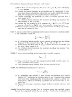
EXAMPLE
I

1.4.
Figure
11.5n
shows the polar plot of an interesting system that has
conditional stability. The system openloop transfer function has the form
Kc(7,,.s
+ I)
GMM(s’GC(s) =
(T,,S
+
i)(T,2S

+

i)(T,j.S

+

l)(Td.S
+ 1)
(

11.23)
If the controller gain
K,.
is such that the
(-

1,O)
point is in the stable region indicated in
Fig. 1 I
.5tr,
the system is closedloop stable. Let us define three values of controller gain:
t
384
PARTTHREE:
Frequency-Domain Dynamics and Control
[m

(G,&)
Stable regions
A
(a) Nyquist plot
Im

(s)

(b) Root locus plot
FIGURE 11.5
System with conditional stability.
K1
= value of K, when 1
GMcjw,
,Gc(io,, 1 = 1
K2
= value of
KC
when IGM(iqjGC(iq)/ = 1
K3
= value of
KC
when
[G~~~~,,G~~~~,,~
= 1
The system is closedloop stable for two ranges of feedback controller gain:
K, <
K,
and
K2
< K, <
K3
(11.24)
This conditional stability is shown on a root locus plot for this system in Fig.
11.5b.
w
11.1.3 Representation
In Chapter 10 we presented three different kinds of graphs that were used to represent

the frequency response of a system: Nyquist, Bode, and Nichols plots. The Nyquist
stability criterion was developed in the previous section for Nyquist or polar plots.
<*IIAIWK

I I
: t;rcquency-uolnain Analysis
(if
Closedloop Systems
385
The critical point for closedloop stability was shown to be the (- I, 0) point on the
Nyquist plot.
Naturally we also can show closedloop stability or instability on Bode and
Nichols plots. The
(-
I, 0) point has a phase angle of
-
180” and a magnitude of
unity or a log modulus of 0 decibels. The stability limit on Bode and Nichols plots
(a) Nyquist plot
+10
0
%
d
-10
-20
-30
(b) Bode plot
+10
0
3

4-
-10
-20
I
I
I
I
-770
-IX0 -90
0
8.
degrees
-270
FIGURE 11.6
Stable and unstable
closedloop systems in
Nyquist, Bode, and Nichols
386
PA~TT~~REE:
Frequency-Domain Dynamics and
Control
is therefore the (0 dB,
-
180”) point. At the limit of closedloop stability
L = 0
dB
and
8
=
-

180” (11.25)
The system is closedloop stable if
L<OdB

at8
= -180”
t9>-180”
atL=OdB
Figure 11.6 illustrates stable and unstable closedloop systems on the three types of
plots.
Keep in mind that we are talking about closedloop stability and that we are
studying it by making frequency response plots of the total openloop system trans-
fer function. These log modulus and phase angle plots are for the
openloop
system.
So we could use the terminology
h
and
80
for our Bode and Nichols plots of the
openloop

GM
Gc frequency response plots.
We consider openloop-stable systems most of the time. We show how to deal
with openloop-unstable processes in Section 11.4.
11.2
CLOSEDLOOP SPECIFICATIONS IN THE FREQUENCY DOMAIN
There are two basic types of specifications commonly used in the frequency do-
main. The first type, phase margin and gain margin, specifies how near the

openloop
GM(iwJGc(iw)
polar plot is to the critical (-
1,O)
point. The second type, maximum
closedloop
log
modulus, specifies the height of the resonant peak on the log modu-
lus Bode plot of the closedloop servo transfer function. So keep the apples and the
oranges straight. We make openloop transfer function plots and look at the (-
1,O)
point. We make closedloop servo transfer function plots and look at the peak in the
log modulus curve (indicating an underdamped system). But in both cases we are
concerned with closedloop stability.
These specifications are easy to use, as we show with some examples in Sec-
tion 11.4. They can be related qualitatively to time-domain specifications such as
damping coefficient.
11.2.1 Phase Margin
Phase margin (PM) is defined as the angle between the negative real axis and a
radial line drawn from the origin to the point where the
GMGc
curve intersects the
unit circle. See Fig. 11.7. The definition is more compact in equation form.
PM
=
180”
+ (arg
GMGc)~~~G~I=
1
(11.26)

If the
GMGC
polar plot goes through the (-
1,O)
point, the phase margin is zero. If
the
GMGr

polar
nlot crosses the
ncmtive
renl
auir

tn
the
r;=ht

nfthn

/-

1
fi\

n-l-+

l
hr.
0

,f
e
I-
l.
e
11
CHAITTER
I I: Frequency-Domain Analysis of Closedloop Systems 387
[m

(GMGc)
A
/
/
/
G,G,
plane
I
*
Re (G.&C)
’
Phase margin = PM
_-
’

/’
Unit circle
G,(im~G~~im~’
\
(a) Nyquist plot

(b) Bode plot
I
.PM
0
3
+i
-20
-180
I
I I
-180
0
0,
degrees
FIGURE 11.7
(c) Nichols plot
Phase margin.
phase margin is some positive angle. The bigger the phase margin, the more stable
is the closedloop system. A negative phase margin means an unstable closedloop
system.
Phase margins of around 45” are often used. Figure 11.7 shows how phase mar-
gin is found on Bode and Nichols plots.