Giáo trình robot - Phần 2 pot
Bạn đang xem bản rút gọn của tài liệu. Xem và tải ngay bản đầy đủ của tài liệu tại đây (1.36 MB, 126 trang )
Part I
Preliminaries
Introduction to Part I
The high quality and rapidity requirements in production systems of our
globalized contemporary world demand a wide variety of technological ad-
vancements. Moreover, the incorporation of these advancements in modern
industrial plants grows rapidly. A notable example of this situation, is the
privileged place that robots occupy in the modernization of numerous sectors
of the society.
The word robot finds its origins in robota which means work in Czech.
In particular, robot was introduced by the Czech science fiction writer Karel
ˇ
Capek to name artificial humanoids – biped robots – which helped human
beings in physically difficult tasks. Thus, beyond its literal definition the term
robot is nowadays used to denote animated autonomous machines. These ma-
chines may be roughly classified as follows:
• Robot manipulators
• Mobile robots
⎧
⎪
⎪
⎪
⎨
⎪
⎪
⎪
⎩
Ground robots
Wheeled robots
Legged robots
Submarine robots
Aerial robots
.
Both, mobile robots and manipulators are key pieces of the mosaic that con-
stitutes robotics nowadays. This book is exclusively devoted to robot manip-
ulators.
Robotics – a term coined by the science fiction writer Isaac Asimov – is
as such a rather recent field in modern technology. The good understanding
and development of robotics applications are conditioned to the good knowl-
edge of different disciplines. Among these, electrical engineering, mechanical
engineering, industrial engineering, computer science and applied mathemat-
ics. Hence, robotics incorporates a variety of fields among which is automatic
control of robot manipulators.
4 Part I
To date, we count several definitions of industrial robot manipulator not
without polemic among authors. According to the definition adopted by the
International Federation of Robotics under standard ISO/TR 8373, a robot
manipulator is defined as follows:
A manipulating industrial robot is an automatically controlled, re-
programmable, multipurpose manipulator programmable in three
or more axes, which may be either fixed in place or mobile for use
in industrial automation applications.
In spite of the above definition, we adopt the following one for the prag-
matic purposes of the present textbook: a robot manipulator – or simply,
manipulator – is a mechanical articulated arm that is constituted of links in-
terconnected through hinges or joints that allow a relative movement between
two consecutive links.
The movement of each joint may be prismatic, revolute or a combination
of both. In this book we consider only joints which are either revolute or pris-
matic. Under reasonable considerations, the number of joints of a manipulator
determines also its number of degrees of freedom (DOF ). Typically, a manip-
ulator possesses 6 DOF, among which 3 determine the position of the end of
the last link in the Cartesian space and 3 more specify its orientation.
q
1
q
2
q
3
Figure I.1. Robot manipulator
Figure I.1 illustrates a robot manipulator. The variables q
1
, q
2
and q
3
are referred to as the joint positions of the robot. Consequently, these posi-
tions denote under the definition of an adequate reference frame, the positions
(displacements) of the robot’s joints which may be linear or angular. For ana-
Introduction to Part I 5
lytical purposes, considering an n-DOF robot manipulator, the joint positions
are collected in the vector q, i.e.
2
q :=
⎡
⎢
⎢
⎣
q
1
q
2
.
.
.
q
n
⎤
⎥
⎥
⎦
.
Physically, the joint positions q are measured by sensors conveniently located
on the robot. The corresponding joint velocities
˙
q :=
d
dt
q may also be mea-
sured or estimated from joint position evolution.
To each joint corresponds an actuator which may be electromechanical,
pneumatic or hydraulic. The actuators have as objective to generate the forces
or torques which produce the movement of the links and consequently, the
movement of the robot as a whole. For analytical purposes these torques and
forces are collected in the vector τ , i.e.
τ :=
⎡
⎢
⎢
⎣
τ
1
τ
2
.
.
.
τ
n
⎤
⎥
⎥
⎦
.
In its industrial application, robot manipulators are commonly employed
in repetitive tasks of precision and others, which may be hazardous for human
beings. The main arguments in favor of the use of manipulators in industry
is the reduction of production costs, enhancement of precision, quality and
productivity while having greater flexibility than specialized machines. In ad-
dition to this, there exist applications which are monopolized by robot manip-
ulators, as is the case of tasks in hazardous conditions such as in radioactive,
toxic zones or where a risk of explosion exists, as well as spatial and sub-
marine applications. Nonetheless, short-term projections show that assembly
tasks will continue to be the main applications of robot manipulators.
2
The symbol “:=” stands for is defined as.
1
What Does “Control of Robots” Involve?
The present textbook focuses on the interaction between robotics and electri-
cal engineering and more specifically, in the area of automatic control. From
this interaction emerges what we call robot control.
Loosely speaking (in this textbook), robot control consists in studying how
to make a robot manipulator perform a task and in materializing the results
of this study in a lab prototype.
In spite of the numerous existing commercial robots, robot control design
is still a field of intensive study among robot constructors and research cen-
ters. Some specialists in automatic control might argue that today’s industrial
robots are already able to perform a variety of complex tasks and therefore,
at first sight, the research on robot control is not justified anymore. Never-
theless, not only is research on robot control an interesting topic by itself but
it also offers important theoretical challenges and more significantly, its study
is indispensable in specific tasks which cannot be performed by the present
commercial robots.
As a general rule, control design may be divided roughly into the following
steps:
• familiarization with the physical system under consideration;
• modeling;
• control specifications.
In the sequel we develop further on these stages, emphasizing specifically
their application in robot control.
8 1 What Does “Control of Robots” Involve?
1.1 Familiarization with the Physical System under
Consideration
On a general basis, during this stage one must determine the physical variables
of the system whose behavior is desired to control. These may be temperature,
pressure, displacement, velocity, etc. These variables are commonly referred to
as the system’s outputs. In addition to this, we must also clearly identify those
variables that are available and that have an influence on the behavior of the
system and more particularly, on its outputs. These variables are referred to
as inputs and may correspond for instance, to the opening of a valve, voltage,
torque, force, etc.
Figure 1.1. Freely moving robot
Figure 1.2. Robot interacting with its environment
In the particular case of robot manipulators, there is a wide variety of
outputs – temporarily denoted by y – whose behavior one may wish to control.
1.1 Familiarization with the Physical System under Consideration 9
For robots moving freely in their workspace, i.e. without interacting with
their environment (cf. Figure 1.1) as for instance robots used for painting,
“pick and place”, laser cutting, etc., the output y to be controlled, may cor-
respond to the joint positions q and joint velocities
˙
q or alternatively, to the
position and orientation of the end-effector (also called end-tool).
For robots such as the one depicted in Figure 1.2 that have physical contact
with their environment, e.g. to perform tasks involving polishing, deburring of
materials, high quality assembling, etc., the output y may include the torques
and forces f exerted by the end-tool over its environment.
Figure 1.3 shows a manipulator holding a marked tray, and a camera which
provides an image of the tray with marks. The output y in this system may
correspond to the coordinates associated to each of the marks with reference
to a screen on a monitor. Figure 1.4 depicts a manipulator whose end-effector
has a camera attached to capture the scenery of its environment. In this case,
the output y may correspond to the coordinates of the dots representing the
marks on the screen and which represent visible objects from the environment
of the robot.
Image
Camera
Figure 1.3. Robotic system: fixed camera
From these examples we conclude that the corresponding output y of a
robot system – involved in a specific class of tasks – may in general, be of the
form
y = y(q,
˙
q, f) .
On the other hand, the input variables, that is, those that may be modified
to affect the evolution of the output, are basically the torques and forces
τ applied by the actuators over the robot’s joints. In Figure 1.5 we show
10 1 What Does “Control of Robots” Involve?
Camera
Image
Figure 1.4. Robotic system: camera in hand
the block-diagram corresponding to the case when the outputs are the joint
positions and velocities, that is,
y = y(q,
˙
q, f)=
q
˙
q
while τ is the input. In this case notice that for robots with n joints one has,
in general, 2n outputs and n inputs.
ROBOT
✲
✲
✲
˙
Figure 1.5. Input–output representation of a robot
1.2 Dynamic Model
At this stage, one determines the mathematical model which relates the input
variables to the output variables. In general, such mathematical representa-
tion of the system is realized by ordinary differential equations. The system’s
mathematical model is obtained typically via one of the two following tech-
niques.
1.2 Dynamic Model 11
• Analytical: this procedure is based on physical laws of the system’s motion.
This methodology has the advantage of yielding a mathematical model as
precise as is wanted.
• Experimental: this procedure requires a certain amount of experimental
data collected from the system itself. Typically one examines the system’s
behavior under specific input signals. The model so obtained is in gen-
eral more imprecise than the analytic model since it largely depends on
the inputs and the operating point
1
. However, in many cases it has the
advantage of being much easier and quicker to obtain.
On certain occasions, at this stage one proceeds to a simplification of the
system model to be controlled in order to design a relatively simple con-
troller. Nevertheless, depending on the degree of simplification, this may yield
malfunctioning of the overall controlled system due to potentially neglected
physical phenomena. The ability of a control system to cope with errors due to
neglected dynamics is commonly referred to as robustness. Thus, one typically
is interested in designing robust controllers.
In other situations, after the modeling stage one performs the parametric
identification. The objective of this task is to obtain the numerical values of
different physical parameters or quantities involved in the dynamic model. The
identification may be performed via techniques that require the measurement
of inputs and outputs to the controlled system.
The dynamic model of robot manipulators is typically derived in the an-
alytic form, that is, using the laws of physics. Due to the mechanical nature
of robot manipulators, the laws of physics involved are basically the laws of
mechanics.
On the other hand, from a dynamical systems viewpoint, an n-DOF system
may be considered as a multivariable nonlinear system. The term “multivari-
able” denotes the fact that the system has multiple (e.g. n) inputs (the forces
and torques τ applied to the joints by the electromechanical, hydraulic or
pneumatic actuators) and, multiple (2n) state variables typically associated
to the n positions q, and n joint velocities
˙
q . In Figure 1.5 we depict the cor-
responding block-diagram assuming that the state variables also correspond
to the outputs. The topic of robot dynamics is presented in Chapter 3. In
Chapter 5 we provide the specific dynamic model of a two-DOF prototype of
a robot manipulator that we use to illustrate through examples, the perfor-
mance of the controllers studied in the succeeding chapters. Readers interested
in the aspects of dynamics are invited to see the references listed on page 16.
As was mentioned earlier, the dynamic models of robot manipulators are
in general characterized by ordinary nonlinear and nonautonomous
2
differ-
ential equations. This fact limits considerably the use of control techniques
1
That is the working regime.
2
That is, they depend on the state variables and time. See Chapter 2.
12 1 What Does “Control of Robots” Involve?
tailored for linear systems, in robot control. In view of this and the present
requirements of precision and rapidity of robot motion it has become neces-
sary to use increasingly sophisticated control techniques. This class of control
systems may include nonlinear and adaptive controllers.
1.3 Control Specifications
During this last stage one proceeds to dictate the desired characteristics for
the control system through the definition of control objectives such as:
• stability;
• regulation (position control);
• trajectory tracking (motion control);
• optimization.
The most important property in a control system, in general, is stabil-
ity. This fundamental concept from control theory basically consists in the
property of a system to go on working at a regime or closely to it for ever.
Two techniques of analysis are typically used in the analytical study of the
stability of controlled robots. The first is based on the so-called Lyapunov sta-
bility theory. The second is the so-called input–output stability theory. Both
techniques are complementary in the sense that the interest in Lyapunov the-
ory is the study of stability of the system using a state variables description,
while in the second one, we are interested in the stability of the system from
an input–output perspective. In this text we concentrate our attention on
Lyapunov stability in the development and analysis of controllers. The foun-
dations of Lyapunov theory are presented in the Chapter 2.
In accordance with the adopted definition of a robot manipulator’s output
y, the control objectives related to regulation and trajectory tracking receive
special names. In particular, in the case when the output y corresponds to the
joint position q and velocity
˙
q, we refer to the control objectives as “position
control in joint coordinates” and “motion control in joint coordinates” respec-
tively. Or we may simply say “position” and “motion” control respectively.
The relevance of these problems motivates a more detailed discussion which
is presented next.
1.4 Motion Control of Robot Manipulators
The simplest way to specify the movement of a manipulator is the so-called
“point-to-point” method. This methodology consists in determining a series
of points in the manipulator’s workspace, which the end-effector is required
1.4 Motion Control of Robot Manipulators 13
to pass through (cf. Figure 1.6). Thus, the position control problem consists
in making the end-effector go to a specified point regardless of the trajectory
followed from its initial configuration.
Figure 1.6. Point-to-point motion specification
A more general way to specify a robot’s motion is via the so-called (con-
tinuous) trajectory. In this case, a (continuous) curve, or path in the state
space and parameterized in time, is available to achieve a desired task. Then,
the motion control problem consists in making the end-effector follow this
trajectory as closely as possible (cf. Figure 1.7). This control problem, whose
study is our central objective, is also referred to as trajectory tracking control.
Let us briefly recapitulate a simple formulation of robot control which, as
a matter of fact, is a particular case of motion control; that is, the position
control problem. In this formulation the specified trajectory is simply a point
in the workspace (which may be translated under appropriate conditions into
a point in the joint space). The position control problem consists in driving the
manipulator’s end-effector (resp. the joint variables) to the desired position,
regardless of the initial posture.
The topic of motion control may in its turn, be fitted in the more general
framework of the so-called robot navigation. The robot navigation problem
consists in solving, in one single step, the following subproblems:
• path planning;
• trajectory generation;
• control design.
14 1 What Does “Control of Robots” Involve?
Figure 1.7. Trajectory motion specification
Path planning consists in determining a curve in the state space, connect-
ing the initial and final desired posture of the end-effector, while avoiding
any obstacle. Trajectory generation consists in parameterizing in time the so-
obtained curve during the path planning. The resulting time-parameterized
trajectory which is commonly called the reference trajectory, is obtained pri-
marily in terms of the coordinates in the workspace. Then, following the so-
called method of inverse kinematics one may obtain a time-parameterized
trajectory for the joint coordinates. The control design consists in solving the
control problem mentioned above.
The main interest of this textbook is the study of motion controllers and
more particularly, the analysis of their inherent stability in the sense of Lya-
punov. Therefore, we assume that the problems of path planning and trajec-
tory generation are previously solved.
The dynamic models of robot manipulators possess parameters which de-
pend on physical quantities such as the mass of the objects possibly held by
the end-effector. This mass is typically unknown, which means that the values
of these parameters are unknown. The problem of controlling systems with
unknown parameters is the main objective of the adaptive controllers. These
owe their name to the addition of an adaptation law which updates on-line,
an estimate of the unknown parameters to be used in the control law. This
motivates the study of adaptive control techniques applied to robot control.
In the past two decades a large body of literature has been devoted to the
adaptive control of manipulators. This problem is examined in Chapters 15
and 16.
We must mention that in view of the scope and audience of the present
textbook, we have excluded some control techniques whose use in robot mo-
Bibliography 15
tion control is supported by a large number of publications contributing both
theoretical and experimental achievements. Among such strategies we men-
tion the so-called passivity-based control, variable-structure control, learning
control, fuzzy control and neural-networks-based. These topics, which demand
a deeper knowledge of control and stability theory, may make part of a second
course on robot control.
Bibliography
A number of concepts and data related to robot manipulators may be found
in the introductory chapters of the following textbooks.
• Paul R., 1981, “Robot manipulators: Mathematics programming and con-
trol”, MIT Press, Cambridge, MA.
• Asada H., Slotine J. J., 1986, “Robot analysis and control ”, Wiley, New
York.
• Fu K., Gonzalez R., Lee C., 1987, “Robotics: Control, sensing, vision and
intelligence”, McGraw–Hill.
• Craig J., 1989, “Introduction to robotics: Mechanics and control”, Addison-
Wesley, Reading, MA.
• Spong M., Vidyasagar M., 1989, “Robot dynamics and control”, Wiley,
New York.
• Yoshikawa T., 1990, “Foundations of robotics: Analysis and control”, The
MIT Press.
• Nakamura Y., 1991, “Advanced robotics: Redundancy and optimization”,
Addison–Wesley, Reading, MA.
• Spong M., Lewis F. L., Abdallah C. T., 1993, “Robot control: Dynamics,
motion planning and analysis”, IEEE Press, New York.
• Lewis F. L., Abdallah C. T., Dawson D. M., 1993, “Control of robot
manipulators”, Macmillan Pub. Co.
• Murray R. M., Li Z., Sastry S., 1994, “A mathematical introduction to
robotic manipulation”, CRC Press, Inc., Boca Raton, FL.
• Qu Z., Dawson D. M., 1996, “Robust tracking control of robot manipula-
tors”, IEEE Press, New York.
• Canudas C., Siciliano B., Bastin G., (Eds), 1996, “Theory of robot con-
trol”, Springer-Verlag, London.
• Arimoto S., 1996, “Control theory of non–linear mechanical systems”, Ox-
ford University Press, New York.
• Sciavicco L., Siciliano B., 2000, “Modeling and control of robot manipula-
tors”, Second Edition, Springer-Verlag, London.
16 1 What Does “Control of Robots” Involve?
• de Queiroz M., Dawson D. M., Nagarkatti S. P., Zhang F., 2000,
“Lyapunov–based control of mechanical systems”, Birkh¨auser, Boston, MA.
Robot dynamics is thoroughly discussed in Spong, Vidyasagar (1989) and
Sciavicco, Siciliano (2000).
To read more on the topics of force control, impedance control and hy-
brid motion/force see among others, the texts of Asada, Slotine (1986), Craig
(1989), Spong, Vidyasagar (1989), and Sciavicco, Siciliano (2000), previously
cited, and the book
• Natale C., 2003, “Interaction control of robot manipulators”, Springer,
Germany.
• Siciliano B., Villani L., “Robot force control”, 1999, Kluwer Academic
Publishers, Norwell, MA.
Aspects of stability in the input–output framework (in particular, passivity-
based control) are studied in the first part of the book
• Ortega R., Lor´ıa A., Nicklasson P. J. and Sira-Ram´ırez H., 1998, “Passivity-
based control of Euler-Lagrange Systems Mechanical, Electrical and Elec-
tromechanical Applications”, Springer-Verlag: London, Communications
and Control Engg. Series.
In addition, we may mention the following classic texts.
• Raibert M., Craig J., 1981, “Hybrid position/force control of manipu-
lators”, ASME Journal of Dynamic Systems, Measurement and Control,
June.
• Hogan N., 1985, “Impedance control: An approach to manipulation. Parts
I, II, and III”, ASME Journal of Dynamic Systems, Measurement and
Control, Vol. 107, March.
• Whitney D., 1987, “ Historical perspective and state of the art in robot
force control”, The International Journal of Robotics Research, Vol. 6,
No. 1, Spring.
The topic of robot navigation may be studied from
• Rimon E., Koditschek D. E., 1992, “Exact robot navigation using artificial
potential functions”, IEEE Transactions on Robotics and Automation, Vol.
8, No. 5, October.
Several theoretical and technological aspects on the guidance of manipu-
lators involving the use of vision sensors may be consulted in the following
books.
Bibliography 17
• Hashimoto K., 1993, “Visual servoing: Real–time control of robot manipu-
lators based on visual sensory feedback”, World Scientific Publishing Co.,
Singapore.
• Corke P.I., 1996, “Visual control of robots: High–performance visual ser-
voing”, Research Studies Press Ltd., Great Britain.
• Vincze M., Hager G. D., 2000, “Robust vision for vision-based control of
motion”, IEEE Press, Washington, USA.
The definition of robot manipulator is taken from
• United Nations/Economic Commission for Europe and International Fed-
eration of Robotics, 2001, “World robotics 2001”, United Nation Pub-
lication sales No. GV.E.01.0.16, ISBN 92–1–101043–8, ISSN 1020–1076,
Printed at United Nations, Geneva, Switzerland.
We list next some of the most significant journals focused on robotics
research.
• Advanced Robotics,
• Autonomous Robots,
• IASTED International Journal of Robotics and Automation
• IEEE/ASME Transactions on Mechatronics,
• IEEE Transactions on Robotics and Automation
3
,
• IEEE Transactions on Robotics,
• Journal of Intelligent and Robotic Systems,
• Journal of Robotic Systems,
• Mechatronics,
• The International Journal of Robotics Research,
• Robotica.
Other journals, which in particular, provide a discussion forum on robot con-
trol are
• ASME Journal of Dynamic Systems, Measurement and Control,
• Automatica,
• IEEE Transactions on Automatic Control,
• IEEE Transactions on Industrial Electronics,
• IEEE Transactions on Systems, Man, and Cybernetics,
• International Journal of Adaptive Control and Signal Processing,
• International Journal of Control,
• Systems and Control Letters.
3
Until June 2004 only.
2
Mathematical Preliminaries
In this chapter we present the foundations of Lyapunov stability theory. The
definitions, lemmas and theorems are borrowed from specialized texts and,
as needed, their statements are adapted for the purposes of this text. The
proofs of these statements are beyond the scope of the present text hence, are
omitted. The interested reader is invited to consult the list of references cited
at the end of the chapter. The proofs of less common results are presented.
The chapter starts by briefly recalling basic concepts of linear algebra
which, together with integral and differential undergraduate calculus, are a
requirement for this book.
Basic Notation
Throughout the text we employ the following mathematical symbols:
∀ meaning “for all”;
∃ meaning “there exists”;
∈ meaning “belong(s) to”;
=⇒ meaning “implies”;
⇐⇒ meaning “is equivalent to” or “if and only if”;
→ meaning “tends to” or “maps onto”;
:= and =: meaning “is defined as” and “equals by definition” respectively;
˙x meaning
dx
dt
.
We denote functions f with domain D and taking values in a set R by
f : D→R. With an abuse of notation we may also denote a function by f(x)
where x ∈D.
20 2 Mathematical Preliminaries
2.1 Linear Algebra
Vectors
Basic notation and definitions of linear algebra are the starting point of our
exposition.
The set of real numbers is denoted by the symbol IR. The real numbers are
expressed by italic small capitalized letters and occasionally, by small Greek
letters.
The set of non-negative real numbers, IR
+
, is defined as
IR
+
= {α ∈ IR : α ∈ [0, ∞)}.
The absolute value of a real number x ∈ IR is denoted by |x|.
We denote by IR
n
, the real vector space of dimension n, that is, the set of
all vectors x of dimension n formed by n real numbers in the column format
x =
⎡
⎢
⎢
⎣
x
1
x
2
.
.
.
x
n
⎤
⎥
⎥
⎦
=[x
1
x
2
··· x
n
]
T
,
where x
1
,x
2
, ···,x
n
∈ IR are the coordinates or components of the vector x
and the super-index
T
denotes transpose. The associated vectors are denoted
by bold small letters, either Latin or Greek.
Vector Product
The inner product of two vectors x, y ∈ IR
n
is defined as
x
T
y =
n
i=1
x
i
y
i
=[x
1
x
2
··· x
n
]
⎡
⎢
⎢
⎣
y
1
y
2
.
.
.
y
n
⎤
⎥
⎥
⎦
=
⎡
⎢
⎢
⎣
x
1
x
2
.
.
.
x
n
⎤
⎥
⎥
⎦
T
⎡
⎢
⎢
⎣
y
1
y
2
.
.
.
y
n
⎤
⎥
⎥
⎦
.
It can be verified that the inner product of two vectors satisfies the following:
• x
T
y = y
T
x for all x, y ∈ IR
n
;
• x
T
(y + z)=x
T
y + x
T
z for all x, y, z ∈ IR
n
.
Euclidean Norm
The Euclidean norm x of a vector x ∈ IR
n
is defined as
2.1 Linear Algebra 21
x :=
n
i=1
x
2
i
=
√
x
T
x,
and satisfies the following axioms and properties:
•x = 0 if and only if x = 0 ∈ IR
n
;
•x > 0 for all x ∈ IR
n
with x = 0 ∈ IR
n
;
•αx = |α|x for all α ∈ IR and x ∈ IR
n
;
•x−y≤x + y≤x + y for all x, y ∈ IR
n
;
•
x
T
y
≤xy for all x, y ∈ IR
n
(Schwartz inequality).
Matrices
We denote by IR
n×m
the set of real matrices A of dimension n ×m formed by
arrays of real numbers ordered in n rows and m columns,
A = {a
ij
} =
⎡
⎢
⎢
⎣
a
11
a
12
··· a
1m
a
21
a
22
··· a
2m
.
.
.
.
.
.
.
.
.
.
.
.
a
n1
a
n2
··· a
nm
⎤
⎥
⎥
⎦
.
A vector x ∈ IR
n
may be interpreted as a particular matrix belonging to
IR
n×1
=IR
n
. The matrices are denoted by Latin capital letters and occasion-
ally by Greek capital letters.
The transpose matrix A
T
= {a
ji
}∈IR
m×n
is obtained by interchanging
the rows and the columns of A = {a
ij
}∈IR
n×m
.
Matrix Product
Consider the matrices A ∈ IR
m×p
and B ∈ IR
p×n
. The product of matrices A
and B denoted by C = AB ∈ IR
m×n
is defined as
C = {c
ij
} = AB
=
⎡
⎢
⎢
⎣
a
11
a
12
··· a
1p
a
21
a
22
··· a
2p
.
.
.
.
.
.
.
.
.
.
.
.
a
m1
a
m2
··· a
mp
⎤
⎥
⎥
⎦
⎡
⎢
⎢
⎣
b
11
b
12
··· b
1n
b
21
b
22
··· b
2n
.
.
.
.
.
.
.
.
.
.
.
.
b
p1
b
p2
··· b
pn
⎤
⎥
⎥
⎦
22 2 Mathematical Preliminaries
=
⎡
⎢
⎢
⎢
⎢
⎢
⎢
⎢
⎢
⎣
p
k=1
a
1k
b
k1
p
k=1
a
1k
b
k2
···
p
k=1
a
1k
b
kn
p
k=1
a
2k
b
k1
p
k=1
a
2k
b
k2
···
p
k=1
a
2k
b
kn
.
.
.
.
.
.
.
.
.
.
.
.
p
k=1
a
mk
b
k1
p
k=1
a
mk
b
k2
···
p
k=1
a
mk
b
kn
⎤
⎥
⎥
⎥
⎥
⎥
⎥
⎥
⎥
⎦
.
It may be verified, without much difficulty, that the product of matrices satisfy
the following:
• (AB)
T
= B
T
A
T
for all A ∈ IR
m×p
and B ∈ IR
p×n
;
• in general, AB = BA;
• for all A ∈ IR
m×p
, B ∈ IR
p×n
:
A(B + C)=AB + AC with C ∈ IR
p×n
;
ABC = A(BC)=(AB)C with C ∈ IR
n×r
.
In accordance with the definition of matrix product, the expression x
T
Ay
where x ∈ IR
n
, A ∈ IR
n×m
and y ∈ IR
m
is given by
x
T
Ay =
⎡
⎢
⎢
⎣
x
1
x
2
.
.
.
x
n
⎤
⎥
⎥
⎦
T
⎡
⎢
⎢
⎣
a
11
a
12
··· a
1m
a
21
a
22
··· a
2m
.
.
.
.
.
.
.
.
.
.
.
.
a
n1
a
n2
··· a
nm
⎤
⎥
⎥
⎦
⎡
⎢
⎢
⎣
y
1
y
2
.
.
.
y
m
⎤
⎥
⎥
⎦
=
n
i=1
m
j=1
a
ij
x
i
y
j
.
Particular Matrices
A matrix A is square if n = m, i.e. if it has as many rows as columns. A square
matrix A ∈ IR
n×n
is symmetric if it is equal to its transpose that is, if A = A
T
.
A is skew-symmetric if A = −A
T
.By−A we obviously mean −A := {−a
ij
}.
The following property of skew-symmetric matrices is particularly useful in
robot control:
x
T
Ax =0, for all x ∈ IR
n
.
A square matrix A = {a
ij
}∈IR
n×n
is diagonal if a
ij
= 0 for all i = j.We
denote a diagonal matrix by diag{a
11
,a
22
, ···,a
nn
}∈IR
n×n
, i.e.
diag{a
11
,a
22
, ···,a
nn
} =
⎡
⎢
⎢
⎣
a
11
0 ··· 0
0 a
22
··· 0
.
.
.
.
.
.
.
.
.
.
.
.
00··· a
nn
⎤
⎥
⎥
⎦
∈ IR
n×n
.
2.1 Linear Algebra 23
Obviously, any diagonal matrix is symmetric. In the particular case when
a
11
= a
22
= ··· = a
nn
= a, the corresponding diagonal matrix is denoted
by diag{a}∈IR
n×n
. Two diagonal matrices of particular importance are the
following. The identity matrix of dimension n which is defined as
I = diag{1} =
⎡
⎢
⎢
⎣
10··· 0
01··· 0
.
.
.
.
.
.
.
.
.
.
.
.
00··· 1
⎤
⎥
⎥
⎦
∈ IR
n×n
and the null matrix of dimension n which is defined as 0
n×n
:= diag{0}∈
IR
n×n
.
A square matrix A ∈ IR
n×n
is singular if its determinant is zero that is,
if det[A]=0. In the opposite case it is nonsingular. The inverse matrix A
−1
exists if and only if A is nonsingular.
A square not necessarily symmetric matrix A ∈ IR
n×n
, is said to be positive
definite if
x
T
Ax > 0, for all x ∈ IR
n
, with x = 0 ∈ IR
n
.
It is important to remark that in contrast to the definition given above, the
majority of texts define positive definiteness for symmetric matrices. However,
for the purposes of this textbook, we use the above-cited definition. This
choice is supported by the following observation: let P be a square matrix of
dimension n and define
A = {a
ij
} =
P + P
T
2
.
The theorem of Sylvester establishes that the matrix P is positive definite if
and only if
det[a
11
] > 0, det
a
11
a
12
a
21
a
22
> 0, ···, det[A] > 0.
We use the notation A>0 to indicate that the matrix A is positive
definite
1
. Any symmetric positive definite matrix A = A
T
> 0 is nonsingular.
Moreover, A = A
T
> 0 if and only if A
−1
=(A
−1
)
T
> 0.
It can also be shown that the sum of two positive definite matrices yields
a positive definite matrix however, the product of two symmetric positive
definite matrices A = A
T
> 0 and B = B
T
> 0, yields in general a matrix
which is neither symmetric nor positive definite. Yet the resulting matrix AB
is nonsingular.
1
It is important to remark that A>0 means that the matrix A is positive definite
and shall not be read as “A is greater than 0” which makes no mathematical
sense.
24 2 Mathematical Preliminaries
A square not necessarily symmetric matrix A ∈ IR
n×n
,ispositive semidef-
inite if
x
T
Ax ≥ 0 for all x ∈ IR
n
.
We employ the notation A ≥ 0 to denote that the matrix A is positive semidef-
inite.
A square matrix A ∈ IR
n×n
is negative definite if −A is positive definite
and it is negative semidefinite if −A is positive semidefinite.
Lemma 2.1. Given a symmetric positive definite matrix A and a nonsingular
matrix B, the product B
T
AB is a symmetric positive definite matrix.
Proof. Notice that the matrix B
T
AB is symmetric. Define y = Bx which, by
virtue of the hypothesis that B is nonsingular, guarantees that y = 0 ∈ IR
n
if and only if x = 0 ∈ IR
n
. From this we obtain
x
T
B
T
AB
x = y
T
Ay > 0
for all x = 0 ∈ IR
n
, which is equivalent to having that B
T
AB is positive
definite. ♦♦♦
Eigenvalues
For each square matrix A ∈ IR
n×n
there exist n eigenvalues (in general, com-
plex numbers) denoted by λ
1
{A},λ
2
{A}, ···,λ
n
{A}. The eigenvalues of the
matrix A ∈ IR
n×n
are numbers that satisfy
det [λ
i
{A}I − A]=0, for i =1, 2, ···,n
where I ∈ IR
n×n
is the identity matrix of dimension n.
For the case of a symmetric matrix A = A
T
∈ IR
n×n
, its eigenvalues are
such that:
• λ
1
{A},λ
2
{A}, ···,λ
n
{A}∈IR ; and,
• expressing the largest and smallest eigenvalues of A by λ
Max
{A} and
λ
min
{A} respectively, the theorem of Rayleigh–Ritz establishes that for
all x ∈ IR
n
we have
λ
Max
{A}x
2
≥ x
T
Ax ≥ λ
min
{A}x
2
.
A symmetric matrix A = A
T
∈ IR
n×n
is positive definite if and only if its
eigenvalues are positive, i.e. if and only if λ
i
{A} > 0 where i =1, 2, ···,n.
Consequently, any square matrix A ∈ IR
n×n
is positive definite if λ
i
{A +
A
T
} > 0 where i =1, 2, ···,n.
2.1 Linear Algebra 25
Remark 2.1. Consider a matrix function A :IR
m
→ IR
n×n
with A symmetric.
We say that A is positive definite if B := A(y) is positive definite for each
y ∈ IR
m
. In other words, if for each y ∈ IR
m
we have
x
T
A(y)x > 0 for all x ∈ IR
n
, with x = 0 .
By an abuse of notation, we define λ
min
{A} as the greatest lower-bound (i.e.
the infimum)ofλ
min
{A(y)} for all y ∈ IR
m
, that is
λ
min
{A} := inf
y ∈IR
m
λ
min
{A(y)}.
For the purposes of this textbook most relevant positive definite matrix func-
tions A :IR
m
→ IR
n×n
satisfy λ
min
{A} > 0.
Spectral Norm
The spectral norm A of a matrix A ∈ IR
n×m
is defined as
2
A =
λ
Max
{A
T
A},
where λ
Max
{A
T
A} denotes the largest eigenvalue of the symmetric matrix
A
T
A ∈ IR
m×m
.
In the particular case of symmetric matrices A = A
T
∈ IR
n×n
,wehave
•A = max
i
|λ
i
{A}|;
•
A
−1
=
1
min
i
|λ
i
{A}|
.
In the expressions above, the absolute value is redundant if A is symmetric
positive definite, i.e. if A = A
T
> 0.
The spectral norm satisfies the following properties and axioms:
•A = 0 if and only if A =0∈ IR
n×m
;
•A > 0 for all A ∈ IR
n×m
where A =0∈ IR
n×m
;
•A + B≤A + B for all A, B ∈ IR
n×m
;
•αA = |α|A for all α ∈ IR and A ∈ IR
n×m
;
•
A
T
B
≤AB for all A, B ∈ IR
n×m
.
2
It is important to see that we employ the same symbol for the Euclidean norm of
a vector and the spectral norm of a matrix. The reader should take special care
in not mistaking them. The distinction can be clearly made via the fonts used for
the argument of ·, i.e. we use small bold letters for vectors and capital letters
for matrices.
26 2 Mathematical Preliminaries
An important result about spectral norms is the following. Consider the
matrix A ∈ IR
n×m
and the vector x ∈ IR
m
. Then, the norm of the vector Ax
satisfies
Ax≤Ax,
where A denotes the spectral norm of the matrix A while x denotes the
Euclidean norm of the vector x. Moreover, since y ∈ IR
n
, the absolute value
of y
T
Ax satisfies
y
T
Ax
≤Ayx.
2.2 Fixed Points
We start with some basic concepts on what are called fixed points; these are
useful to establish conditions for existence and unicity of equilibria for ordi-
nary differential equations. Such theorems are employed later to study closed-
loop dynamic systems appearing in robot control problems. To start with, we
present the definition of fixed point that, in spite of its simplicity, is of great
importance.
Consider a continuous function f :IR
n
→ IR
n
. The vector x
∗
∈ IR
n
is a
fixed point of f (x)if
f(x
∗
)=x
∗
.
According to this definition, if x
∗
is a fixed point of the function f (x),
then x
∗
is a solution of f(x) −x = 0.
Some functions have one or multiple fixed points but there also exist func-
tions which have no fixed points. The function f(x) = sin(x) has a unique
fixed point at x
∗
= 0, while the function f (x)=x
3
has three fixed points:
x
∗
=1,x
∗
= 0 and x
∗
= −1. However, f (x)=e
x
has no fixed point.
We present next a version of the contraction mapping theorem which pro-
vides a sufficient condition for existence and unicity of fixed points.
Theorem 2.1. Contraction Mapping
Consider Ω ⊂ IR
m
, a vector of parameters θ ∈ Ω and the continuous function
f : IR
n
× Ω → IR
n
. Assume that there exists a non-negative constant k such
that for all y, z ∈ IR
n
and all θ ∈ Ω we have
f(y, θ) −f(z, θ)≤k y −z.
If the constant k is strictly smaller than one, then for each θ
∗
∈ Ω, the
function f(·, θ
∗
) possesses a unique fixed point x
∗
∈ IR
n
.
Moreover, the fixed point x
∗
may be determined by
x
∗
= lim
n→∞
x(n, θ
∗
)
where x(n, θ
∗
)=f(x(n −1, θ
∗
)) and with x(0, θ
∗
) ∈ IR
n
being arbitrary.
2.3 Lyapunov Stability 27
An important interpretation of the contraction mapping theorem is the
following. Assume that the function f(x, θ) satisfies the condition of the theo-
rem then, for each θ
∗
∈ Ω the equation f (x, θ
∗
) −x = 0 has a solution in x
and moreover it is unique. To illustrate this idea consider the function h(x, θ)
defined as
h(x, θ)=ax −b sin(θ −x) (2.1)
= −a [f(x, θ) −x]
with a>0, b>0, θ ∈ IR and
f(x, θ)=
b
a
sin(θ −x). (2.2)
We wish to find conditions on a and b so that h(x, θ) = 0 has a unique
solution in x. From (2.1) and (2.2) we see that this is equivalent to establishing
conditions to guarantee that
b
a
sin(θ −x) − x = 0 has a unique solution in x.
In other words, conditions to ensure that
b
a
sin(θ −x) has a unique fixed point
for each θ. To solve this problem we may employ the contraction mapping
theorem. Notice that
|f(y, θ) − f(z, θ)| =
b
a
[sin(θ −y) −sin(θ −z)]
and, invoking the mean value theorem (cf. Theorem A.2 on page 384) which
ensures that |sin(θ − y) − sin(θ −z)|≤|y − z|, we obtain
|f(y, θ) − f(z, θ)|≤
b
a
|y − z|
for all y, z and θ ∈ IR. Hence, if 1 > b/a ≥ 0 for each θ, f(x, θ) has a unique
fixed point and consequently, h(x, θ) = 0 has a unique solution in x.
2.3 Lyapunov Stability
In this section we present the basic concepts and theorems related to Lyapunov
stability and, in particular the so-called second method of Lyapunov or
direct method of Lyapunov.
The main objective in Lyapunov stability theory is to study the behavior
of dynamical systems described by ordinary differential equations of the form
˙
x = f(t, x), x ∈ IR
n
,t∈ IR
+
, (2.3)
where the vector x corresponds to the state of the system represented by
(2.3). We denote solutions of this differential equation by x(t, t
◦
, x(t
◦
)). That
28 2 Mathematical Preliminaries
is, x(t, t
◦
, x(t
◦
)) represents the value of the system’s state at time t and with
arbitrary initial state x(t
◦
) ∈ IR
n
and initial time t
◦
≥ 0. However, for sim-
plicity in the notation and since the initial conditions t
◦
and x(t
◦
) are fixed,
most often we use x(t) to denote a solution to (2.3) in place of x(t, t
◦
, x(t
◦
)).
We assume that the function f :IR
+
× IR
n
→ IR
n
is continuous in t and
x and is such that:
• Equation (2.3) has a unique solution corresponding to each initial condition
t
◦
, x(t
◦
);
• the solution x(t, t
◦
, x(t
◦
)) of (2.3) depends continuously on the initial con-
ditions t
◦
, x(t
◦
).
Generally speaking, assuming existence of the solutions for all t ≥ t
◦
≥ 0is
restrictive and one may simply assume that they exist on a finite interval.
Then, existence on the infinite interval may be concluded from the same the-
orems on Lyapunov stability that we present later in this chapter. However,
for the purposes of this book we assume existence on the infinite interval.
If the function f does not depend explicitly on time, that is, if f (t, x)=
f(x) then, Equation (2.3) becomes
˙
x = f(x), x ∈ IR
n
(2.4)
and it is said to be autonomous. In this case it makes no sense to speak of
the initial time t
◦
since for any given t
◦
and t
◦
such that x(t
◦
)=x(t
◦
), we
have x(t
◦
+ T,t
◦
, x(t
◦
)) = x(t
◦
+ T,t
◦
, x(t
◦
)) for any T ≥ 0. Therefore, for
all autonomous differential equations we can safely consider that t
◦
=0.
If f (t, x)=A(t)x + u(t) with A(t) being a square matrix of dimension
n and A(t) and vector u(t) being functions only of t – or constant – then
Equation (2.3) is said to be linear. In the opposite case it is nonlinear.
2.3.1 The Concept of Equilibrium
Among the basic concepts in Lyapunov theory that we underline are: equi-
librium, stability, asymptotic stability, exponential stability and uniformity.
We develop each of these concepts below. First, we present the concept of
equilibrium which plays a central role in Lyapunov theory.
Definition 2.1. Equilibrium
A constant vector x
e
∈ IR
n
is an equilibrium or equilibrium state of the system
(2.3) if
f(t, x
e
)=0 ∀ t ≥ 0 .
A direct consequence of the definition of equilibrium, under regularity
appropriate conditions that exclude “pathological” situations, is that if the
initial state x(t
◦
) ∈ IR
n
is an equilibrium (x(t
◦
)=x
e
∈ IR
n
) then,