inventory management spare parts and reliability centred maintenance for production lines
Bạn đang xem bản rút gọn của tài liệu. Xem và tải ngay bản đầy đủ của tài liệu tại đây (1.51 MB, 51 trang )
10
Inventory Management, Spare Parts
and Reliability Centred Maintenance
for Production Lines
Fausto Galetto
Politecnico di Torino
Turin
Italy
1. Introduction
1
st
Premise
: Ever since he was a young student, at the secondary school, Fausto Galetto was
fond of understanding the matters he was studying: understanding for learning was his
credo (ϕιλομαθης συνιημι); for all his life he was keeping this attitude, studying more than
one ton of pages: as manager and as consultant he studied several methods invented by
professors, but never he used the (many) wrong ones; on the contrary, he has been devising
many original methods needed for solving the problems of the Companies he worked for,
and presenting them at international conferences [where he met many bad divulgers, also
professors “ASQC certified quality auditors
”]; after 25 years of applications and experience, he
became professor, with a dream “improve future managers (students) quality”: the
incompetents he met since then grew dramatically (also with documents. F.Galetto got from
students ERASMUS
, (Fijiu Antony et al., 2001, Sarin S. 1997). 2
nd
Premise: “The wealth of
nations depends increasingly on the quality of managers.” (A. Jay) and “Universities
grow future
managers.” (F. Galetto) Entailment: due to that, the author with this paper will try, again, to
provide the important consequent message: let's, all of us, be scientific in all Universities, that
is, let's all use our rationality. “What I want to teach is: to pass from a hidden non-sense to a non-
sense clear.” (L. Wittgenstein). END
[see the Galetto references]
“In my university studies …, in most of the cases, it seemed that students were asked simply to
regurgitate at the exams what they had swallowed during the courses.” (M. Gell-Mann “The Quark
and the Jaguar ” [1994]). Some of those students later could have become researchers and
then professors, writing “scientific” papers and books … For these last, another statement of
the Nobel Prize M. Gell-Mann is relevant: “Once that such a misunderstanding has taken place in
the publication, it tends to become perpetual, because the various authors simply copy one each
other.” , similar to “Imitatores, servum pecus” [Horatius, 18 B.C.!!] and “Gravior et validior
est decem virorum bonorum sententia quam totius multitudinis imperitiae” [Cicero]. When
they teach, “The result is that hundreds of people are learning what is wrong
. I make this
statement on the basis of experience, seeing every day the devastating effects of incompetent
teaching and faulty applications. [Deming (1986)]”, because those professors are unable to
practice maieutics [μαιευτικη τεχνη], the way used by Socrates for teaching [the same was
for Galileo Galilei in the Dialogue on the Two Chief World Systems]. Paraphrasing P. B. Crosby,
www.intechopen.com
New Trends in Technologies: Control, Management, Computational Intelligence and Network Systems
160
in his book Quality is free, we could say “Professors may or may not realize what has to be
done to achieve quality. Or worse, they may feel, mistakenly, that they do understand what
has to be done. Those types can cause the most harm.”
What do have in common Crosby, Deming and Gell-Mann statements? The fact that
professors and students betray an important characteristic of human beings: rationality [the
“Adult state” of E. Berne (see fig. 1)]. Human beings are driven by curiosity that demands
that we ask questions (“why?. …, why?”) and we try to put things in order (“this is
connected with that”): curiosity is one of the best ways to learn, but “learning does not mean
understanding”; only twenty-six centuries ago, in Greece, people began to have the idea that
the “world” could be “understood rationally”, overcoming the religious myths: they were
sceptic [σκεπτομαι=to observe, to investigate] and critic [κρινω=to judge]: then and there a
new kind of knowledge arose, the “rational knowledge”.
Till today, after so long time, we still do not use appropriately our brain! A peculiar, stupid
and terrific non-sense! During his deep and long experience of Managing and Teaching
(more than 40 years), F. Galetto always had the opportunity of verifying the truth of Crosby,
Deming and Gell-Mann statements.
Before proceeding we need to define the word “scientific”.
A document (paper or book) is “scientific” if it “scientifically (i.e. with “scientific method”)
deals with matters concerning science (or science principles, or science rules)”. Therefore to
be “scientific” a paper must both concern “science matters” and be in accordance with the
“scientific method”.
The word “science” is derived from the Latin word “scire” (to know for certain) {derived
from the Greek words μαθησις, επιστημη, meaning learning and knowledge, which, at that
time, were very superior to “opinion” [δοξα], while today opinion of many is considered
better than the knowledge of very few!}; knowledge is strongly related to “logic reasoning”
[λογικος νους], as it was, for ages, for Euclid, whose Geometry was considered the best
model of “scientificness”. Common (good) sense
is not science! Common sense does not
look for “understanding”, while science looks for “understanding”! “Understanding” is
related to “intelligence” (from the Latin verb “intelligere” ([intus+legere: read into]:
“intellige ut credas” i.e. understand to believe. Unfortunately “none so deaf as those that won't
hear”.
Let's give an example, the Pythagoras Theorem: In a right triangle, the square of the length of the
hypotenuse equals the sum of the squares of the lengths of the other two sides. Is this statement
scientific? It could be scientific because it concerns the science of Geometry and it can be
proven true by mathematical arguments. It is not-scientific because we did not specify that
we were dealing with the “Euclidean Geometry” (based, among others, on the “parallel
axiom”: from this only, one can derive that the sum of the interior angles of a triangle is
always
π
): we did not deal “scientifically” with the axioms; we assumed them implicitly.
So we see that “scientificness” is present only if the set of statements (concerning a given
“system”) are non-contradictory and deductible from stated principles (as the rules of Logic
and the Axioms).
Let's give another example, the 2
nd
law of Mechanics: The force and the acceleration of a body are
proportional vectors: F=ma, (m is the mass of the body). Is this statement scientific? It could be
scientific because it concerns the science of Mechanics and it can be proven “true” by well
designed experiments. It is not-scientific because we did not specify that we were dealing
with “frames of reference moving relatively one to another with constant velocity” [inertial
www.intechopen.com
Inventory Management, Spare Parts and Reliability Centred Maintenance for Production Lines
161
frames (with the so called “Galilean Relativity”: the laws of Physics look the same for
inertial systems)] and that the speed involved was not comparable with the “speed of light
in the vacuum [that is the same for all observers]” (as proved by the Michelson-Morley
experiment: in the Special Relativity Theory, F=d(mv)/dt is true, not F=ma!) and not
involving atomic or subatomic particles. We did not deal “scientifically” with the
hypotheses; we assumed them implicitly. From the laws of Special Relativity we can derive
logically the conservation laws of momentum and of energy, as could Newton for the
“Galilean Relativity”. For atomic or subatomic particles “quantum Mechanics” is needed
(with Schrödinger equation as fundamental law).
ε
Q
IO
GE
ε
Q
IO
GE
Think
well
to DECIDE
what how when where
MEASURE to DECIDE
Think
well
to DECIDE
what how when where
MEASURE to DECIDE
F. Galetto
F. Galetto
F focus
A assess
U understand
S scientifically
T test
A activate
V verify
I implement
A assure
again and again
again and again
the profitable route to Quality
the profitable route to Quality
Definitions & Hypotheses
LOGIC Deduction
Prediction
Experiments
Matching
Definitions & Hypotheses
LOGIC Deduction
Prediction
Experiments
Matching
Induction
Induction
P
A
C
ε
Q
IO
GE
ε
Q
IO
GE
S C I E N T I F I C N E S S
F. Galetto
F. Galetto
Fig. 1. Scientificness
So we see that “scientificness” is present only
if the set of statements (concerning a given
“system”) do not contradict the observed data, collected through well designed experiments
[“scientific” experiments]: only in the XVII century, due to Galilei, Descartes, Newton, … we
learned that. Since that time only, science could really grow.
When we start trying to learn something, generally, we are in the “clouds”; reality (and
truth) is hidden by the clouds of our ignorance, the clouds of the data, the clouds of our
misconceptions, the clouds of our prejudices; to understand the phenomena we need to find
out the reality from the clouds: we make hypotheses, then we deduct logically some
consequences, predicting the results of experiments: if predictions and experimental data do
match then we “confirm” our idea and if many other are able to check our findings we get a
theory. To generate a theory we need Methods. Eric Berne, the psychologist father of
“Transactional Analysis”, stated that everybody interacts with other people trough three
states P, A, C [Parent, Adult, Child, (not connected with our age, fig. 1)]: the Adult state is
the one that looks for reality, makes questions, considers the data, analyses objectively the
data, draws conclusions and takes logic decisions, coherent with the data, methodically.
Theory [θεωρια] comes from the Adult state! Methods [μεθοδος from μετα+οδος = the way
through (which one finds out…)] used to generate a Theory come from the Adult state!
People who take for granted that the truth depends on “Ipse dixit” [αυτος εϕα, “he said
that”], behave with the Parent state. People who get upset if one finds their errors and they
www.intechopen.com
New Trends in Technologies: Control, Management, Computational Intelligence and Network Systems
162
do not consider them [“we are many and so we are right”, they say!!] behave with the Child
state. [see the books of the Palo Alto group]
To find scientifically the truth (out of the clouds) you must Focus on the problem, Assess
where you are (with previous data and knowledge), Understand Scientifically the message
in the data and find consequences that confirm (or disprove) your predictions, Scientifically
design Test for confirmation (or disproval) and then Activate to make the Tests. If you and
others Verify you prediction, anybody can Implement actions and Assure that the results
are SCIENTIFIC (FAUSTA VIA): all of us then have a THEORY. SCIENTIFICNESS is there
(fig. 1).
From these two examples it is important to realise that when two people want to verbally
communicate, they must have some common concepts, they agree upon, in order to transfer
information and ideas between each other; this is a prerequisite, if they want to understand
each other: what is true for them, what is their “conventional” meaning of the words they
use, which are the rules to deduce statements (Theses) from other statements (Hypotheses
and “previous” Theses): rigour is needed for science
, not opinions!!!
Many people must apply Metanoia [μετανοια=change their mind (to understand)] to find the
truth.
Here we accept the rules of LOGIC, the deductive logic, where the premises of a valid
argument contain the conclusion, and the truth of the conclusion follows from the truth of
the premises with certainty: any well-formed sentence is either true or false. We define as
Theorem “a statement that is proven true by reasoning, according to the rules of Logic”; we
must therefore define the term True: “something” (statement, concept, idea, sentence,
proposition) is true when there is correspondence between the “something” and the facts,
situations or state of affairs that verify it; the truth is a relation of coherence between a thesis
and the hypotheses. Logical validity is a relationship between the premises and the
conclusion such that if the premises are true then the conclusion is true. The validity of an
argument should be distinguished from the truth of the conclusion (based on the premises).
This kind of truth is found in mathematics.
Human beings evolved because they were able to develop their knowledge from inside (the
deductive logic, with analytic statements) and from outside, the external world, (the inductive
logic, with synthetic statements), in any case using their intelligence
; the inductive logic is
such that the premises are evidence for the conclusion, but the truth of the conclusion
follows from the truth of the evidence only with a certain probability, provided the way of
reasoning is correct.
The scientific knowledge is such that any valid knowledge claim must be verifiable in
experience and built up both through the inductive logic (with its synthetic statements) and
the deductive logic (with its analytic statements); in any case a clear distinction must be
maintained between analytic and synthetic statements.
This was the attitude of Galileo Galilei in his studies of falling bodies. At first time he
formulated the tentative hypothesis that “the speed attained by a falling body is directly
proportional to the distance traversed”; then he deduced from his hypothesis the conclusion
that objects falling equal distances require the same amount of elapsed time. After
“Gedanken Experimenten”, Designed Experiments made clear that this was a false
conclusion: hence, logically
, the first hypothesis had to be false. Therefore Galileo framed a
new hypothesis: “the speed attained is directly proportional to the time elapsed”. From this
he was able to deduce that the distance traversed by a falling object was proportional to the
www.intechopen.com
Inventory Management, Spare Parts and Reliability Centred Maintenance for Production Lines
163
square of the time elapsed; through Designed Experiments, by rolling balls down an
inclined plane, he was able to verify experimentally his thesis (it was the first formulation of
the 2
nd
law of Mechanics). [fig. 1]
Such agreement of a conclusion with an actual observation does not itself prove the
correctness of the hypothesis from which the conclusion is derived. It simply renders that
premise much more plausible.
For rational people
(like were the ancient Greeks) the criticism [κρινω = to judge] is hoped
for, because it permits improvement: asking questions, debating and looking for answers
improves our understanding: we do not know the truth, but we can look for it and be able to
find it, with our brain; to judge we need criteria [κριτεριον]. In this search Mathematics
[note μαθησις] and Logic can help us a lot: Mathematics and Logic are the languages that
Rational Managers must know! Proposing the criterion of testability, or falsificability, for
scientific validity, Popper emphasized the hypothetico-deductive character of science. Scientific
theories are hypotheses from which can be deduced statements testable by observation; if
the appropriate experimental observations falsify these statements, the hypothesis is
refused. If a hypothesis survives efforts to falsify it, it may be tentatively accepted. No
scientific theory, however, can be conclusively established. A “theory” that is falsified, is
NOT scientific.
“Good theories” are such that they complete previous “good” theories, in accordance with
the collected new data. [fig. 1]
A good example of that is Bell's Inequality. In physics, this inequality was used to show
that a class of theories that were intended to “complete” quantum mechanics, namely local
hidden variable theories, are in fact inconsistent with quantum mechanics; quantum
mechanics typically predicts probabilities, not certainties, for the outcomes of
measurements. Albert Einstein [one of the greatest scientists] stated that quantum
mechanics was incomplete, and that there must exist “hidden” variables that would make
possible definite predictions. In 1964, J. S. Bell proved that all local hidden variable theories
are inconsistent with quantum mechanics, first through a “Gedanken Experiment” and
Logic, and later through Designed Experiments. Also the great scientist, A. Einstein, was
wrong in this case: his idea was falsified. We see then that the ultimate test of the validity of
a scientific hypothesis is its consistency with the totality of other aspects of the scientific
framework. This inner consistency constitutes the basis for the concept of causality in
science, according to which every effect is assumed to be linked with a cause. [fig. 1]
The scientific community as a whole must judge [κρινω] the work of its members by the
objectivity and rigour with which that work has been conducted; in this way the scientific
method should prevail.
In any case the scientific community must remember: Any statement (or method) that is
falsified, is NOT scientific.
Here we assume
that the subject of a paper is concerning a science (like Mathematics,
Statistics, Probability, Quality Methods); therefore to judge [κρινω] if a paper is scientific we
have to look at the “scientific method”: if the “scientific method” is present, i.e. the
conclusions (statements)
in the paper follow logically from the hypotheses, we shall
consider the paper scientific; on the contrary, if there are conclusions (statements) in the
paper that do not follow logically from the hypotheses, we shall NOT consider the paper
scientific: a wrong conclusion (statement) is NOT scientific
. [fig. 1 vs Franceschini 1999]
“To understand that an answer is wrong you don't need exceptional intelligence, but to understand
that is wrong a question one needs a creative mind.” (A. Jay). “Intellige ut credas”.
www.intechopen.com
New Trends in Technologies: Control, Management, Computational Intelligence and Network Systems
164
Right questions, with right methods, have to be asked to “ nature” (fig. 1).
“Intellige ut credas”.
It is easy
to show that a paper, a book, a method, is not scientific: it is sufficient to find an
example that proves the wrongness of the conclusion. When there are formulas in a paper, it
is not necessary to find the right formula to prove that a formula is wrong: an example is
enough; to prove that a formula is wrong, one needs only intelligence; on the contrary, to
find the right formula, that substitutes the wrong one, you need both intelligence and
ingenuity. I will use only intelligence and I will not give any proof of my ingenuity: this
paper is for intelligence … For example, it's well known (from Algebra, Newton identities)
that the coefficients and the roots of any algebraic equation are related: it's easy to prove that
ac /−±
is not the solution (even if you do not know the right solution) of the parabolic
equation
0
2
=++ cbxax
, because the system x
1
+ x
2
= -b/a , x
1
x
2
= c/a is not satisfied (x
1
and
x
2
are the roots). [Montgomery 1996 and ]
The literature on “Quality” matters is rapidly expanding. Unfortunately, nobody, but me, as
far as I know, [I thank any person that will send me names of people who take care …],
takes care of the Quality of Quality Methods used for making Quality
(of product,
processes and services). “Intellige ut credas”. [O' Connor 1997, Brandimarte 2004]
I am eager to meet one of them, fond of Quality as I am. [fig. 1, and Galetto references]
If this kind of person existed, he would have agreed that “facts and figures are useless, if not
dangerous, without a sound theory” (F. Galetto), “Management need to grow-up their
knowledge because experience alone, without theory, teaches nothing what to do to make
Quality” (Deming) because he had seen, like Deming, Gell-Mann and myself “The result is
that hundreds of people are learning what is wrong
. I make this statement on the basis of
experience, seeing every day the devastating effects of incompetent teaching and faulty
applications.” [Deming (1986)] (Montgomery 1996 and , Franceschini 1999)
During 2006 F. Galetto experienced the incompetence of several people who were thinking
that only the “Peer Review Process” is able to assure the scientificness of papers, and that
only papers published in some magazines are scientific: one is a scientist and gets funds if
he publishes on those magazines!!! Using the scientific method one can prove that the
referee analysis does not assure quality of publications in the magazines of fig. 2.
A
P
C
A
P
C
F focus
A assess
U understand
S scientifically
T test
A activate
V verify
I implement
A assure
again and again
again and again
the profitable route to Quality
the profitable route to Quality
ε
Q
IO
GE
ε
Q
IO
GE
F. Galetto
F. Galetto
F. Galetto
F. Galetto
ε
Q
IO
GE
ε
Q
IO
GE
Fig. 2. The “pentalogy”
www.intechopen.com
Inventory Management, Spare Parts and Reliability Centred Maintenance for Production Lines
165
The symbol
IO
GE
Q
ε
[which stands for the “epsilon Quality”] was devised by F. Galetto to
show that Quality depends, at any instant, in any place, at any rate of improvement, on the
Intellectual hOnesty of people who always use experiments and think well on the
experiments before actually making them (Gedanken Experimenten) to find the truth”
[Gedanken Experimenten was a statement used by Einstein; but, if you look at Galileo life, you
can see that also the Italian scientist was used to “mental experiments”, the most important
tool for Science; Epsilon (
ε) is a greek letter used in Mathematics and Engineering to indicate
a very small quantity (actually going to zero); epsilon Quality conveys the idea that Quality
is made of many and many prevention and improvement actions].
The level of knowledge F. Galetto could verify (in 40 years experience and a lot of meetings)
is given in table 1.
Logic
Management
Mathematics
Physics
Quality Management
Probability
Stochastic Processes
Statistics
Applied Statistical Methods
Parameter Estimation
Test of Hypotheses
Decision Making
System Reliability Theory
Maintainability
Design Of Experiments
Control Charts
Sampling Plans
Quality Engineering
Quality Practice
Professors
1
H
VL
95
VL
98
VL
98
VL
99
VL
99
VL
99
VL
99
VL
99
VL
99
VL
99
VL
95
VL
99
VL
99
VL
99
VL
99
VL
99
VL
99
VL
99
Managers
VL
95
VL
95
VL
98
VL
98
VL
99
VL
99
VL
99
VL
99
VL
99
VL
99
VL
99
VL
95
VL
99
VL
99
VL
99
VL
99
VL
99
1
VH
1
VH
Consultants
VL
99
VL
95
VL
98
VL
98
VL
99
VL
99
VL
99
VL
99
VL
99
VL
99
VL
99
VL
95
VL
99
VL
99
VL
99
VL
99
VL
99
1
VH
1
VH
Legenda : VL90=probability 90% that knowledge is lower than Very Low;
5VH=probability 5% that knowledge is higher than Very High
Scale: None, Very Low, Low, Medium, High, Very High, Perfect
Table 1. Level of Knowledge (based on 40 year of experience, in companies and universities)
Many times F. Galetto spoiled his time and enthusiasm at conferences, in University and in
Company courses, trying to provide good ideas on Quality and showing many cases of
wrong applications of stupid methods [see references]. He will try to do it again … by
showing, step by step, very few cases (out of the hundreds he could document) in order
people understand that QUALITY is a serious matter. The Nobel price R. Feynman (1965)
said that
for the progress of Science are necessary experimental capability, honesty in providing the
results and the intelligence of interpreting them… We need to take into account of the experiments
even though
the results are different from our expectations. It is apparent that Deming and
Feynman and Gell-Mann are in agreement with
IO
GE
Q
ε
ideas of F. Galetto. Once upon a time,
A. Einstein said “Surely there are two things infinite in the world: the Universe and the Stupidity of
people. But I have some doubt that Universe is infinite”. Let's hope that Einstein was wrong, this
time. Anyway, before him, Galileo Galilei had said [in the Saggiatore] something similar
“Infinite is the mob of fools “. [see references]
www.intechopen.com
New Trends in Technologies: Control, Management, Computational Intelligence and Network Systems
166
All the methods, devised by F. Galetto, were invented and have been used for preventing
and solving real problems in the Companies he was working for, as Quality Manager and as
Quality Consultant: several million € have been saved.[see Galetto references]
Companies will not be able to survive the global market if they cannot provide integrally
their customer the Quality they have paid for [fig. 5, Management Tetrahedron]. So it is of
paramount importance to define correctly what Quality means. Quality is a serious and
difficult business; it has to become an integral part of management.
The first step is to define
logically what Quality is.
Let's start with some ideas of Soren Bisgard (2005) given in the paper Innovation, ENBIS and
the Importance of Practice in the Development of Statistics, Quality and Reliability
Engineering International. He says: “Since the early 1930s industrial statistics has been almost
synonymous with quality control and quality improvement. Some of the most important innovations
in statistical theory and methods have been associated with quality.” …. “Quality Management also
provides an intriguing example. Its scientific underpinning is greatly inspired by statistics, a point
forcefully set forth by Shewhart. Quality is typically interpreted narrowly by statisticians as variance
and defect reduction. However these efforts should be viewed more broadly as what economist call
innovation. When we engage in statistical quality control studies … we are engaged in process
innovation and … in product innovation.” Two paragraphs of his paper are entitled: 2.
Quality as innovation, and 3. Quality as systematic innovation.
One must say that the paper does not provide the definition of the term Quality, such as
“Quality is …”; however he realises that statisticians have a narrow view of Quality, as
“Quality is variance and defect reduction
.”
As a matter of fact, D. C. Montgomery defines: “Quality is the inverse of variability” (saying
“We prefer a modern definition of quality”) and adds “Quality Improvement is the reduction of
variability in processes and products”. To understand the following subject the reader has to
know Reliability and Statistics. Let's consider two computers (products A and B): after 3
years, A experiences g
A
(3)=9 failures, while B experiences g
B
(3)=5 failures; which product
has better quality? B, because it experienced less failures! BUT, which product has lower
variability? A, because it experienced more failures!
Generally, statisticians (and professors) do not understand this point: they are Gauss-
drugged with the “normal distribution”! Let's assume, for the sake of simplicity, that two
items have constant increasing failure rate (IFR, they do wear and do not have infant
mortality); form the data we can estimate the MTTF (Mean Time To Failure), the Reliability
R(t) and the probability density of failures f(t): B is more reliable and has more variability
[the upper curve]! Therefore according to D. C. Montgomery definition B (that is more
reliable) has lower “quality”! Fig 3 provides a hint for understanding ….
0
0.2
0.4
0.6
0.8
1
1.2
0
20
40
60
80
100
120
140
160
180
200
220
240
260
280
300
Reliability
time
Fig. 3. An item with more variability B, has better Quality
www.intechopen.com
Inventory Management, Spare Parts and Reliability Centred Maintenance for Production Lines
167
If one thinks to the Formula One Championship and applies Montgomery's definition he
finds that if the two Red Bull arrive 1
st
and 2
nd
they have lower quality than the two Ferrari
that arrive 7
th
and 8
th
!!!!! Can you believe it?
There are a lot of “quality definitions; let's see some of the latest definitions of the word
“Quality” that can be found in the literature (some of them existed before the date here
given; the date shown refers to the latest document I read):
“conformance to requirements” (Crosby, 1979), “fitness for use” (Juran ,1988), “customer
satisfaction” (Juran, 1993), “the total composite product and service characteristics of
marketing, engineering, manufacture and maintenance through which product or service in
use will meet the expectations by the customer” (Feigenbaum, 1983 and 1991)¸“totality of
characteristics of an entity that bears on its ability to satisfy stated and implied needs” (ISO
8402:1994), “a predictable degree of uniformity and dependability at low cost and suited to the
market” (falsely
attributed to Deming, 1986; I read again and again Deming documents and I
could not find that), “Quality is inversely proportional to variability” (Montgomery, 1996),
“degree to which a set of inherent characteristics (3.5.1) fulfils requirements (3.1.2)” [ISO
9000:2000, Quality management systems – Fundamentals and vocabulary, (definition 3.1.1)]
The ISO definition is very stupid; it is like confounding two very different concepts: energy
and temperature; “temperature” provides the
degree of “energy” [=Quality]; therefore
Quality must be “the set of characteristics”.
Quality definition must have Quality in it!
In order to provide a practical and managerial definition, since 1985 F. Galetto was
proposing the following one:
Quality is the set of characteristics of a system that makes it able to satisfy the needs of
the Customer, of the User and of the Society. It is clear that none of the previous eight
definitions highlights the importance of the needs of the three actors: the Customer, the
User and the Society. They are still not considered in the latest document, the ISO
9000:2008, Quality management systems – Fundamentals and vocabulary.
Some important characteristics are stated in the Quality Tetrahedron of ten characteristics
Safety, Conformity, Reliability, Durability, Maintainability, Performance, Service, Aesthetics,
Economy, Ecology; each characteristic has an “operational definition” that permits to state
goals and verify achievement [according to FAUSTA VIA]. “Customer/User/Society
needs
satisfaction” must be converted from a slogan to real practice, if companies want to be
competitive. Today, many managers show their commitment with customer satisfaction, but
they are not prepared to invest time and money in NEEDS Satisfaction; they do not put the
theory into practice; they do not speak with the facts, but only with words.
Unfortunately
management commitment to Quality is not enough
; managers must understand
and learn Quality ideas: too many companies are well behind the desired level of Quality
management practices. [fig. 5]
The Quality Tetrahedron shows that Management must learn that solving problems is
essential but it is not enough: they must prevent future problems and take preventive
actions: Safety, Reliability, Durability, Maintainability, Ecology, Economy can be tackled
rightly only through preventive actions; the PDCA cycle is useless for prevention; it very
useful for improvement. Several of the Quality characteristics [in the Quality Tetrahedron]
need prevention; reliability is one of the most important: very rarely failures can be
attributed to blue collar workers. Failures arise from lack of prevention, and prevention is a
fundamental aspect and responsibility of Management. The same happens for safety,
durability, maintainability, ecology, economy,
www.intechopen.com
New Trends in Technologies: Control, Management, Computational Intelligence and Network Systems
168
Service
Aesthetics Ecology Economy
DurabilityMaintainability
Reliability
Conformity
Performance
Safety
Quality Tetrahedron
F. Galetto
Fig. 4. The Quality Tetrahedron for the Quality definition
So we see that Quality entails much more than “innovation”: you can innovate without
Quality! Few decades ago electronic gadgets entered into cars; electronics was an innovation
in cars, but the cars failed a lot: innovation did not take into consideration prevention! The
essence of Quality is prevention. Innovation is a means for competition, rarely for Quality.
(see the “Business Management System” in figure 5).
We are in a new economic age: long-term thinking, prevention, Quality built at the design
stage, understanding variation, waste elimination, knowledge and scientific approach are
concepts absolutely needed by Management , if they want to be good Managers. In this
paper, Manager is the person who
achieves the Company goals, economically, through other
people, recognise existing problems, prevents future problems, states priorities, dealing with their
conflicts, makes decisions thinking to their consequences, with rational and scientific method, using
thinking capability and knowledge of people. These kind of Managers behave according to the
“Business Management System”.
The customer is the most important driving force of any company. Companies will not be
able to survive the global market if they cannot provide integrally their customer the
Quality they have paid for. It is important to stress that “Customer Needs Satisfaction” is
absolutely different from “Customer Satisfaction”. Moreover, the previous analysis show
that for a good definition of Quality there are other people involved: the user and the
Society.
Prevention We said that the essence of Quality is prevention. Innovation is a means for
competition, rarely for Quality. (see the “Business Management System”). Quality is
essential for any product (services are defined as products in the ISO 9000:2000
terminology). The measurement of Quality (of product and services) is important if we want
to improve and better if we want to prevent problems [F. Galetto from 1973]. Quality
depends on effective management of problems prevention and correction (improvement).
Effective management needs effective measurement of performance and results, the
absolute condition to achieve Business Excellence. A Company that wants to become
“excellent” has to find the needs of Customers/Users/Society and to measure how much
they are achieved. Moreover that Company has to be “sure” that all its processes are “in
www.intechopen.com
Inventory Management, Spare Parts and Reliability Centred Maintenance for Production Lines
169
Q
Prevention
Prevention
Quality Essence
( the core is Prevention )
Corrective Action
• F. Galetto
• F. Galetto
QUALITY
INTEGRITY
INTELLECTUAL HONESTY
HOLISTIC
COOPERATION and
CLIMATE
MANGEMENT TETRAHEDRON
SCIENTIFIC APPROACH to DECISIONS ( M B I T E )
• F. Galetto
• F. Galetto
COMPETITIVENESS TETRAHEDRON
• F. Galetto
• F. Galetto
RATIONAL MANAGER TETRAHEDRON
DECISIONS
ANALYSIS
KNOWLEDGE LOGIC
THEORY (M B I T E )
PREVENTION
ANALYSIS
PROBLEMS
ANALYSIS
• F. Galetto
• F. Galetto
Corrective
Corrective
ActionAction
R
e
s
p
o
n
s
e
Spee
d
P
r
o
f
i
t
a
b
i
l
i
t
y
P
r
i
c
e
I
m
a
g
e
I
n
n
o
v
a
t
i
o
n
Q
u
a
l
i
t
y
ε
Q
GE
IO
ε
Q
GE
IO
ε
Q
GE
IO
ε
Q
GE
IO
Fig. 5. The Business Management System
Customer/User
Society
Needs
Preliminary
Specifications
Design
Pre-production Production Field
PREVENTIVE
Actions
CORRECTIVE Actions
and
Product Improvement
Q U A L I T Y
Development Cycle
•F. Galetto
Product
Specifications
Testing
Design
Testing
ε
Q
IO
GE
ε
Q
IO
GE
ε
Q
IO
GE
ε
Q
IO
GE
ε
Q
IO
GE
ε
Q
IO
GE
Correttive
Q
Prevenzione
Prevenzione
Essenza della Qualità
(il nucleo è la Prevenzione)
Correttive
CorrettiveAzioni
Azioni
Azioni
• F. Galetto
WORK
PEOPLE
$$$ $$$
£££ £££
T Q M
2
T
estify
Q
uality
of
M
anagement in
M
anagement
• effectiveness •responsiveness
• efficiency
Estetica
Ecologia Economicità
Service
Conformità
Durata
Affidabilità
Sicurezza
Tetraedro della Qualità
• F. Gale tto
Prestazioni
Manutenibilità
ε
Q
IO
GE
Tetraedro delle 10 Aree Chiave
Verifiche di
Produz ione
Preproduzione Fornitori
Controllo di
Processo
Progetta zione
Esigenze dei
Cli enti ,
Utilizzatori,
Soci età
Miglioramenti
Sistema
Informativo
Sperimentazione
Organi zzazione
• F. Gal etto
Fig. 6. The Development Cycle
www.intechopen.com
New Trends in Technologies: Control, Management, Computational Intelligence and Network Systems
170
control”. If data are available (through properly designed method of collection), statistical
methods are the foundation stone for good data analysis and “management decisions” [F.
Galetto from 1973].
Prevention is very important and must be considered since from the first stages of product
development as shown in figure 6; corrective actions come later.
Reliability is important in all the stages of product development. Reliability tests are
essential during product development; collected data have to be analysed by scientific
methods that involve Engineering, Statistics and Probability Methods. Reliability is
important for preventive maintenance and for the so called RCM (Reliability Centred
Maintenance). Let's for example consider the methods for data analyses and maintenance
planning, as given in the papers “Total time on test plotting for failure data analyses
”,
(1978), SAAB-SCANIA, and “Some graphical methods for maintenance planning
”, (1977),
Reliability & Maintainability Symposium. They are connected with similar ideas of Barlow.
Let' consider a sample made of n “identical” items (n=sample size), that are neither repaired
nor replaced after failure. We can view the tested sample as a system (“in parallel”) that can
be represented as in the graph, where state “i” indicates that “i” items are failed; g indicates
the last failure observed during the test. When g=n we can apply the TTT-plot.
g-1 g01
At any time instant x, some of the n units can be still alive
(survived up to time x), while the other are failed, before x; the sum of all the “survival
times” of the n items put on test is denoted TTT(x) [and named the Total Time on Test, up to
the time instant x]; the duration of the test depends on the failure of the last item (out of the
n) that will fail. If the items fail at times t
1
, t
2
, …, t
n
, then TTT(t
1
) is the Total Time on Test
until the 1
st
failure, TTT(t
i
) is the Total Time on Test until the i
th
failure and TTT(t
n
) is the
Total Time on Test until the i
th
failure. If T
i
is the random variable “Time to the i
th
failure” then
TTT(T
i
) is the random variable “Total Time on Test until the i
th
failure”: the distribution of the
random variable TTT(T
i
) depends on the distribution of the random variable T
i
, which depends
on the distribution of the random variable T “Time to Failure” of any of the n “identical”
items put on test. The n-1 random variables U
i
=TTT(T
i
)/TTT(T
n
), the scaled TTT, have a
distribution that depends on the random variable T “Time to Failure” of any item; since the
distribution F
T
(t) of the r.v. T depends on the failure rate, one can plot a curve F
U
(t) [named
TTT-transform] versus F
T
(t): the curve is contained in the square unit of the Cartesian plane
and its shape depends on the type of the failure rate [constant, IFR (increasing), or DFR
(decreasing)]. Therefore the TTT-plotting allows understanding the type of failure rate.
The evolution of the system depends from the functions b
i,i+1
(s|r)ds, probability of the
transition i⇒i+1 (i.e. the (i+1)
th
failure) in the interval s
s+ds, given that it happened into
the state “i” at the time instant r; the functions b
i,i+1
(s|r) [named “kernel of the stochastic
process” of failures] (Galetto, ….) allow to get the probability
(|)
i
Wtr
that the system
remains in the state i for the period r
t and the probability R
i
(t|r) [reliability relative to state
i] that the system does not be in the state g at time t (given that it entered in i at time instant
r). R
0
(t|0) is then the probability that the system, in the interval 0
t, does not reach the state
g, i.e. it experienced less than g failures: G(t)<g. We have then the fundamental system of
Integral Theory of Estimates [valid for any distribution of time to failure of tested units, i.e. for
any “kernel”]
,1 1 1,
( | ) ( | ) ( | ) ( | ) ,i=0,
g
-1 e ( | ) 0
t
ii iii gg
r
Rtr Wtr b srR tsds b sr
++ −
=
+=
∫
www.intechopen.com
Inventory Management, Spare Parts and Reliability Centred Maintenance for Production Lines
171
For g=n we get the probability of n failures 1- R
0
(t|0) and the Total Time on Test.
If the items on test have constant failure rate λ, then b
i,i+1
(s|r) = nλ exp[-nλ(s-r)], when failed
items are replaced or repaired, while b
i,i+1
(s|r) = (n-i)λ exp[-(n-i)λ(s-r)], when failed items
are not
replaced or repaired.
After the test one has the data. Let's suppose n=7 and the time to failure (in the sample) are
60, 105, 180, 300, 400, 605, 890. One can estimate F
U
(t
i
) and F
T
(t
i
), and plot the 7 points
[F
U
(t
i
),F
T
(t
i
)], obtaining the “empirical” curve.
Now Statistics Theory enters the stage. When the reliability of the items is exponential
(constant failure rate), the TTT-transform F
U
(t) versus F
T
(t) is the diagonal of the unit square
(the bisector of the coordinate axes). Plotting the “empirical” curve. [F
U
(t
i
),F
T
(t
i
)] one finds a
line “near” the bisector (β=1), and concludes that a constant failure rate is adequate. When
the reliability of the items is IFR, the TTT-transform F
U
(t) versus F
T
(t) is a convex curve
above the diagonal of the unit square. Figure 7 provides some curves depending on the
“shape parameter β“.
To practitioners this can be fantastic. They collect data, elaborate them and then they
compare the “empirical” curve with the “Theoretical Curve” given in figure 7; then they
“
know” the failure distribution and take decisions. Perhaps the situation is more complex ….
• And … what you do if you do not have the figure 7? Are you able to generate it?
• Now let's suppose that we, as managers, decide to save time for decision and we
replace
the items failed and we continue the test. Can we use the same figure 7?
• Now let's suppose that we, as managers, decide to save time for decision and we repair
the items failed and we continue the test. Can we use the same figure 7?
• Now let's suppose that we, as managers, decide to save time for decision and we test
more items (e.g. 28) and we stop the test at the 7
th
failure. Can we use the same figure 7?
• Now let's suppose that we, as managers, decide to save time for decision and we test
more items (e.g. 50) and we stop the test at the time instant t=200. Can we use the same
figure 7?
IF one is a sensible Manager
he will answer: “I do not know. I have to study a lot; I have also
to be careful if I go to some consultant”. IF one is a NOTsensible Manager
he will answer:
“Yes, absolutely”.
Let's see now how a problem is dealt in the paper “Total time on test plotting for failure data
analyses”; in Section 5 “SYSTEM FAILURE DATA” we read [verbatim] “It is also possible to
use the TTT-plotting technique for analysing failure data from a repairable system. In this case
TTT(T
i
) shall be defined as the time generated by the system until the i
th
failure. If n-1 failures have
been obtained until time T*, the time during which the system was observed, then we substitute T* to
T
n
and perform the plotting as before. Also the interpretation of the plot remains unchanged. The
TTT-transform has, however, no counterpart. The statistical tests described in Section 4 are still
applicable.” [end of Section]. In Section 4 “STATISTICAL TESTS” we read [verbatim] “Based
on the ideas behind the TTT-plotting some statistical test may be obtained. These tests also provides
us with some insight in the stochastic properties of the TTT-plot. ……. “
Now let’s use Logic, as we said before. IF The TTT-transform
does not exist how can one
consider “The statistical tests described in Section 4 are still applicable.”? They are “Based on the
ideas behind the TTT-plotting …” which “has, however, no counterpart
.” !!!! From the TTT-plot
one can only have some hints of the non-applicability of “constant failure rate”!!! Nothing
more! Moreover, IF one does not know TTT-transform for repairable systems, he should say
“I do not know how to find the TTT-transform” and not “
The TTT-transform has, however, no
counterpart.”
www.intechopen.com
New Trends in Technologies: Control, Management, Computational Intelligence and Network Systems
172
TTT-transform of Weibull Reliability
0
0,1
0,2
0,3
0,4
0,5
0,6
0,7
0,8
0,9
1
0 0,1 0,2 0,3 0,4 0,5 0,6 0,7 0,8 0,9 1
FT(t)
FU(t
)
1 2 3 3,6
0,8 0,65 0,5 0,3333
Fig. 7. Weibull TTT-transform [with “shape parameter β“]
As a matter of fact, in 1977, at the Reliability & Maintainability Symposium, Philadelphia, F.
Galetto provided the Reliability Integral Theory that solves the problem, with his paper
“SARA (System Availability and Reliability Analysis)”. The theory did exist, not the single
formulae: any scholar could have found them. The same theory Reliability Integral Theory,
is applicable to maintenance problems, as those presented in “Some graphical methods for
maintenance planning”; we will deal with this point in a successive paragraph related to
preventive maintenance.
2. Logistics and inventory
Inventories are stockpiles of raw material, supplies, components, work in progress and
finished goods that appear at numerous points throughout a firm's production and logistic
channel. Having these inventories on hand cost at least 20% of their value per year,
therefore, carefully managing inventory levels makes good economic sense, because in
recent years the holding of inventories has been roundly criticised as unnecessary end
wasteful. Actually good management of inventories improve customer service and reduce
costs. Inventory plays a key role in the logistical behaviour of all manufacturing systems.
The classical inventory results are central to more modern techniques of manufacturing
management, such as material requirement planning (MRP), just-in-time (JIT) and time
based competition (TBC).
1
st
step: the case of “constant (fixed)” demand
Let's consider the oldest, and simplest,
model – the Economic Order Quantity – in order to work our way to the more sophisticated
ReOrder Level (ROL) model. One of the earliest applications of mathematics to factory
www.intechopen.com
Inventory Management, Spare Parts and Reliability Centred Maintenance for Production Lines
173
management was the work of F. W. Harris (1913) on the problem of setting manufacturing
lot sizes. He made the following assumptions about the manufacturing system: 1)
production is instantaneous, 2) delivery is immediate, 3) a production run incurs a fixed
setup cost, 4) there is no interaction between different products, 5) demand is deterministic,
6) demand is constant over time.
Let's consider the problem of establishing the order quantity Q [lot size] for an inventory
system, dealt in “Logistics courses” and related books. In this field the assumptions are very
similar: a single item is subject to “constant (fixed)” demand “λ“ [demand rate, in units per
year], there is a fixed cost A [ordering cost, in euro] of placing an order and a carrying
charge “h” [holding cost, in euro per unit per unit time allotted (often year) to each item in
inventory]. If no stockouts are permitted and lead time is zero (i.e. orders arrive
immediately) there is a quantity Q (named EOQ: Economic Order Quantity), given by the
famous Wilson lot-size formula
2/QAh
λ
= that minimise the “total cost per year”. The
inventory can be depicted as a system that starts with Q units (the level, I, of the inventory):
we are certain that λt units are sold (delivered) in any interval of duration t; when the level
inventory is zero, I=0, Q products are ordered and arrive immediately and the system
starts again from scratch.
Fig. 8. System inventory states, with fixed and constant demand; state i means i products
dispatched
The function depicting the curve of the inventory level I(t) is a saw-tooth line, with constant
distance between peaks.
Fig. 9. Level of inventory versus time t
The production cost does not influence the solution and therefore in not considered in the
“total cost per year” Y(Q)= hQ/2+Aλ/Q. Taking the derivative of Y(Q), and using
elementary concepts of calculus, one gets easily the Wilson formula
2/QAh
λ
=
. In this
particular case, I repeat, in this particular case, the number of lots ordered per year is
N=λ/Q and the optimal time between orders is T=Q/λ, i.e. T=1/N.
Let's now see what happened in a MASTER (after 5 years of Engineering courses) on
Maintenance and Reliability, in the lessons for RCM [Reliability Centred Maintenance]:
www.intechopen.com
New Trends in Technologies: Control, Management, Computational Intelligence and Network Systems
174
Wilson formula
2/QAh
λ
= , which holds only in the hypotheses we said just before, was
provided to student for buying the spare parts, which obviously depend on the number of
failures, which obviously depend on the unreliability, which obviously depend on the time
failure, which obviously is a random variable!!! A serious teacher should have proved that
the formula holds true, before teaching it to students !!!!
2
nd
step: the case of random demand with “constant” demand rate and steady state of the
stochastic process We are going now to consider the demand as a random variable, so
introducing the need of the use of probability theory. If we maintain all the previous
hypotheses, but the number 5 and 6: 1) production is instantaneous, 2) delivery is
immediate, 3) a production run incurs a fixed setup cost, 4) there is no interaction between
different products, 5) demand is random
, 6) demand rate is constant over time. We can depict the
system as before [and in fig. 10]
Fig. 10. System inventory states, with random demand and constant demand rate; state i
means i products dispatched
where now the “time to sell a new unit (time between demands)” is a random variable
exponentially distributed.
The function depicting the curve of the inventory level I(t) is a saw-tooth line, with variable
[randomly] time distance between peaks.
Fig. 11. Level of inventory versus time t
Therefore the probabilistic structure of the inventory system is a Markov process, periodic
with period Q. The mean time (holding time) in any state is m=1/λ, the steady-state
transition probability from one state i, to the next state i-1 is constant ϕ
i
= ϕ
i-1
= 1/Q [use
Markov chains theory]. The “reward structure” is such that the order cost A is associated
with the transition from state Q-1 to 0, while the holding cost, per unit time, for state i is y
i
=
(Q-i)*h, i=2 to Q, and y
1
= h+λA; the average cost per unit time, g (cost rate), for operating
the system in the steady state is
(1)/2/
g
AhQQ Q
λ
=+ +
⎡⎤
⎣⎦
The value Q that optimise the cost rate, in the steady state of the stochastic process, i.e. when
the time is tending to infinity, is found as the solution of the previous equation. If Q is large,
we can ignore the discrete nature of Q [Q is an integral number], assuming it can be
www.intechopen.com
Inventory Management, Spare Parts and Reliability Centred Maintenance for Production Lines
175
considered as a continuous variable: so we can differentiate and set the derivative equal to
zero; the solution is (the famous Wilson lot-size formula)
hAQ /2
λ
=
. If Q is small, we
cannot ignore the discrete nature of Q [Q is an integral number], and the solution has to be
find numerically.
3
rd
: the case of random demand with “variable” demand rate and steady state of the
stochastic process We are going to consider again the demand as a random variable, (need
probability theory), maintaining all the previous hypotheses [as in the 2
nd
case], but the
number 6, : 1) production is instantaneous, 2) delivery is immediate, 3) a production run
incurs a fixed setup cost, 4) there is no interaction between different products, 5)
demand is
random, 6) demand rate is NOT constant over time, but it varies with time, identically after any
transition from a state to the following one.
We can depict, again, the system as before [and in fig. 12]
Fig. 12. System inventory states, with random demand and variable demand rate; state i
means i products dispatched
where now the “time to sell a new unit (time between demands)” is a random variable
“identically” [but not exponentially] distributed; let indicate the probability density of the
time between transitions as f(t) [related to the “rate” λ(t), with cumulative distribution F(t)];
its mean is m.
The mean number of state transitions in the interval 0
t, M(t) is the solution of the integral
equation
0
() () () ( )
t
M
tFt frMtrdr=+ −
∫
(1)
The related intensity of state transitions, at time t, is m(t)=dM(t)/dt, the solution of the
integral equation
0
() () () ( )
t
mt f t f rmt rdr=+ −
∫
(2)
In the process steady state we have M(t)≅t/m and m(t) )≅1/m, for t → ∞. The function
depicting the curve of the inventory level I(t) is a saw-tooth line, with variable [randomly]
time distance between peaks, too. [fig. 13]
Therefore the probabilistic structure of the inventory system is a semi-Markov process,
periodic with period Q. The mean time (holding time) in any state is m [the mean of the
distribution] identical for all the states; then the steady-state transition probability from one
state i, to the next state i-1 is constant ϕ
i
= ϕ
i-1
= 1/Q [use semi-Markov processes theory].
The “reward structure” is such that the order cost A is associated with the transition from
www.intechopen.com
New Trends in Technologies: Control, Management, Computational Intelligence and Network Systems
176
Fig. 13. Level of inventory versus time t
state Q-1 to 0, while the holding cost, per unit time, for state i is y
i
= (Q-i)*h, i=2 to Q, and y
1
= h+A/m; the average cost per unit time, g (cost rate), for operating the system in the steady
state is the same, as before, / ( 1) /2 /
g
AmhQQ Q=++
⎡⎤
⎣⎦
.
The value Q that optimise the cost rate, in the steady state of the stochastic process, i.e. when
the time is tending to infinity, is found as the solution of the previous equation. If Q is large,
we can ignore the discrete nature of Q [Q is an integral number], assuming it can be
considered as a continuous variable: so we can differentiate and set the derivative equal to
zero; the solution is
2/( )QAmh= (similar to the famous Wilson lot-size formula); if
different types of distributions are used, but with the same mean, one gets the same
optimum g. If Q is small, we cannot ignore the discrete nature of Q [Q is an integral
number], and the solution has to be find numerically.
Notice that we can manipulate the formula, obtaining the following
(1)/2AhmQQ
g
mQ mQ
+
=+ that shows very clearly a fundamental fact of renewal processes:
the gain rate, in the steady state of a process
, is the ratio of the cost during a renewal cycle
and the length of the cycle [mQ, that is the mean sum of Q random variables, identically
distributed]; we will find the same idea in the formulae of preventive maintenance.
Notice that nobody says that the formulas in the various books and papers are to be
considered only for the steady state
.
It is very interesting noting that, after a long time t
*
, at which the stochastic process reaches
“almost surely” its steady state, the cost for the interval t
*
t
*
+t is
1
/(1)/2gt At m Q Q ht
Q
=++
⎡
⎤
⎣
⎦
(3)
which shows that t/m is the mean number of orders for the interval t
*
t
*
+t (in the steady
state) and Q(Q+1)ht/2 is the mean number of products, for holding which we pay, for the
interval t
*
t
*
+t (in the steady state).
4
th
step: the case of random demand with “constant” demand rate and steady state of the
stochastic process We are going to consider the demand as a random variable, so
introducing the need of the use of probability theory, but we consider a lead time different
from 0, we maintain some of the previous hypotheses, but the number 2, 5 and 6: 1)
production is instantaneous, 2) delivery takes a constant time L, named Lead Time, after the
order, 3) a production run incurs a fixed setup cost, 4) there is no interaction between
different products, 5) demand is random, 6) demand rate is constant over time. We can no longer
depict the system as before; we need to distinguish between the net inventory I(t) and the
inventory position IP(t). The net inventory I(t) is the actual number of products we have on
hand that we can send to our customers, after a time L, form their order. The inventory
www.intechopen.com
Inventory Management, Spare Parts and Reliability Centred Maintenance for Production Lines
177
position IP(t) is the sum of I(t), the actual number of products we have on hand, the
outstanding orders not yet arrived at time t, minus the products backlogged.; the order of Q
products is placed, at any time t
0
, when IP(t
0
) equals the ROL (the Re-Order Level);
unfortunately, in the meantime [duration L] a stockout might occur: while we wait for the
lot arrival (replenishment of the inventory), at time t
0
+ L, the net inventory I(t) and the
inventory position IP(t) decrease because of selling (and dispatching) products. If it happens
that I(t
STO
)=0, at a time t
STO
, we face an inventory STockOut, that generates a cost: customers
are unsatisfied ; we lose to sell products, a case named “Lost Sales”. The cost involved in
this case are: the order cost A, the cost of holding the inventory (that varies with time), and
the “penalty cost” due to stockout. The “time to sell a new unit (time between demands)” is
a random variable exponentially distributed. The function depicting the curve of the
Inventory Position level IP(t) is a saw-tooth line, with variable [randomly] time distance
between peaks, exponentially distributed. [fig. 14]
Fig. 14. Level of the inventory position versus time t
Therefore the probabilistic structure of the inventory system is a Markov process, periodic
with period Q. The mean time (holding time) in any state is m=1/λ, the steady-state
transition probability from one state IP=i, to the next state IP=i-1, in the process steady state,
is still constant ϕ
i
= ϕ
i-1
= 1/Q [use Markov chains theory and fig. 15].
Fig. 15. System inventory states, with random demand and constant demand rate; state i
means i products dispatched
www.intechopen.com
New Trends in Technologies: Control, Management, Computational Intelligence and Network Systems
178
The “reward structure” is such that the order cost A is associated with the transition from
state Q+ROL and ROL; the carrying inventory cost is associated with the mean number of
products on hand times the time they are in the inventory, while the stockout cost is related
to the probability that happens the event I(t)=0, in spite that we have ROL product when we
order the lot of Q products. [we will use, for short, R for the ROL, ReOrder Level]
Let t
0
be the time instant when IP(t
0
)=R; the net inventory I(t
0
+L) = R - demanded quantity
X
L
, during the lead time L, is a random variable with the same type of distribution as
Inventory Position IP(t
0
+L);, for any interval t
0
t
0
+Δt the holding cost is a random variable
as well
0
0
00
() ( )
tt
t
h I u du hTTI t t t
+Δ
−−−−
=
+Δ
∫
(4)
where we name “total time of inventory”, TTI(t
0
t
0
+Δt), for any interval t
0
t
0
+Δt, the
time for which we have to pay for the products we have on hands [net inventory ] and for
the time they are on hands.
The mean of this random variable is
0
0
00
[ ( )] [ ( )]
tt
t
h E I u du hE TTI t t t
+Δ
−−−−
=
+Δ
∫
(5)
Being I(t)=IP(t)-Q, for any time t, the “total time of inventory”, TTI(t
0
t
0
+Δt) depends on
the transitions between the states 0, 1, 2, , Q and the related probabilities. Therefore the
mean of TTI is
{}
00
[ ( )] ( ) ( 1) ( 1) ( 1)
t
ETTIt t t R Q R Q R Q R Q t
λ
−−−−
Δ
+
Δ= + + +−+ +−++ + −Δ
(6)
Using simple concepts of Algebra, we get
{}
00
[( )] ( )( 1)(1) /
2
t
ETTIt t t R Q R Q RR Q t
λ
λ
λ
−−−−
Δ
+Δ = + + + − + − Δ
(7)
Letting T
Q
be the random time for selling Q products, and so reorder a new lot of products,
we have, for any planning cycle t
0
t
0
+ T
Q
{}
00
[( )] ( 1)/2
Q
Q
ETTIt t T R Q L
λ
λ
−−−−
+= ++ −
(8)
Therefore the expected cost of inventory is
{}
(1)/2
Q
hRQ L
λ
λ
++ −
(9)
We proved this formula using probability theory; in all the books I read never there was the
proof! Why?
The quantity ss=R - λL is the safety stock that we hold in order to prevent stockouts.
www.intechopen.com
Inventory Management, Spare Parts and Reliability Centred Maintenance for Production Lines
179
If t
0
is the time instant when IP(t
0
)=R; the stockout happens when the net inventory I(t
0
+L) =
R - demanded quantity X
L
, during the lead time L, which is a random variable, falls below
zero: P
STO
=P[I(t
0
+L) ≤0]; it means that, at some instant, t
STO
≤ t
0
+L, I(t
0
+ t
STO
) =0. Letting T
R
be the random time for selling R product, we have P
STO
=P[T
R
≤ L].
If T
R
> L the system is able to provide products, we have on hand (net inventory), to all
customers asking for them, filling their demands; that’s why the probability S(R,L) = P[T
R
>
L] = 1-P
STO
, is named Service Level (type 1), or Fill Rate.
Noting that P[T
R
> L] is the “reliability of a stand-by system of R products” failing with
failure rate equal to λ, one can take advantage of the use of all the ideas of Reliability Theory
for the field of Inventory Management.
Here we are doing that.
Let T
STO
be the random variable “Time To Stock Out” of the inventory system and N
STO
(t) be
the random variable “Number of Stock Outs” of the system, in the interval 0
t; at time t
the system has a “residual life” ρ(t) until the next Stock Out,
()
()
STO
Nt
tT t
ρ
=
− ; since the
transitions depend on the exponential distribution ρ(t) is independent from the Number of
the experienced Stockouts. Let S(R, t+x| t) = P[ρ(t) > x] be the type 1 Service Level, related to
the interval t
t+x; F. Galetto proved [chapter 6 of Affidabilità, Volume 1: Teoria e Metodi di
Calcolo, (1995) CLEUP, Padova. Italy] that the type 1 Service Level S(R,t+x|t) = P[ρ(t) > x] is
the solution of the integral equation
0
(, |) (, |0) ()(, |)
t
STO
SRt x t SRt x f sSRt x sds+= ++ +
∫
(10)
where f
STO
(t) is the probability density function of the 1
st
T
STO
, with mean denoted as
MTTSTO and named Mean Time To STockOut.
If t→∞ the type 1 Service Level S(R,t+x|t) depends only on x; F. Galetto proved [chapter 6 of
Affidabilità, Volume 1: Teoria e Metodi di Calcolo, (1995) CLEUP, Padova. Italy] that S(R, x) =
P[ρ(∞) > x] is related to the density of stock outs f
STO
(x|∞)= S(R, x|0)/MTTSTO.
Therefore, after a long time t that the inventory system is running, the steady state type 1
Service Level S(R, L) is
(,) (,)
L
SRL SRsds
∞
=
∫
(11)
3. What one can find in documents
The following excerpts are copied directly from books; it is not important to report the
names of the authors! None of the authors say that their formulae hold only in the steady
state of the process. Notice that a lot of attention is needed in order to find the
correspondence between the different notations.
From a book one can find, where d is the random demand, LT is the lead time, F
dLT
(R) is the
cumulative probability of sales during LT, p is the cost (penalty) of stock out. Notice that
there is no proof of this formula in the book.
www.intechopen.com
New Trends in Technologies: Control, Management, Computational Intelligence and Network Systems
180
From another book one can find, where CSL is the Cycle Service Level [i.e. the fraction of
replenishment cycles that end with all customer demand being met (a replenishment cycle is
the interval between two successive replenishment deliveries). The CSL is equal to the
probability of not having a stockout in a replenishment cycle, H is the cost of holding one
item for one unit of time, C
u
is the cost of one item, D is the average demand for one unit of
time.
In the notations of the previous book D
L
=E(d), H=h, ROP=R, replenishment cycle is equal
LT, CSL is then F
dLT
(R), ss=R - λL (safety stock).
From another book, again, one can find, where G(r)=S(Q, r) is the Service Level (type 1), I(Q,
r) is the average net inventory, D is the expected demand per year (in units), k is the cost per
stockout.
In the notations of the previous book D=D
L
=E(d), h=H=h, r=ROP=R, S(Q, r)=CSL=F
dLT
(R),
k=p.
Notice that that the three books provide to the students (or the managers) three different
formulae for the same concept, the type 1 Service Level!!!
www.intechopen.com
Inventory Management, Spare Parts and Reliability Centred Maintenance for Production Lines
181
Book
Formula for Service
Level
Equivalence only IF Equivalence only IF
1 F
dLT
(R)
F
dLT
(R) = 1 - HQ/(HQ
+DC
u
)
F
dLT
(R) = kD/(kD + hQ)
2
CSL = 1 - HQ/(HQ
+DC
u
)
DC
u
= kD
1 - HQ/(HQ +DC
u
) =
F
dLT
(R)
3 G(r) = kD/(kD + hQ) kD/(kD + hQ) = F
dLT
(R) kD = DC
u
It is very clear that it is very improbable that the cost per stockout is equal to the cost per
unit.
A case from Fctory Physics
www.intechopen.com
New Trends in Technologies: Control, Management, Computational Intelligence and Network Systems
182
Let’s provide clearly the relevant data: annual demand D=14. NOTICE “estimated from
historical data”, without any confidence interval!, Lead time L = 45 days cost of order A = 15
$, holding cost h = 30 $ per unit per year stockout cost k= 40 $, demand distribution:
Poisson. Since the demand distribution is Poisson, the time between demand is
exponentially distributed, and the system can be modelled with a Markov chain in the
steady state of the process.
On the contrary, the Factory Physics authors “approximate the Poisson by the normal, with mean
1.726 and standard deviation
σ
=1.314”; then they compute Q=3.7 (≅4) and r=2.946 (≅3) [with
the formula G(r) = kD/(kD + hQ)].
Using “reliability theory”, we draw the transition diagram, with transition (selling) rate λ
[solid lines] and replenishment [dotted lines]; in the steady state we can write the steady
transition probability matrix P that provides us with the MTTSTO, the Cost per Unit Time,
the Service Level. We compared our findings with the ones of the Factory Physics authors
who “approximate the Poisson by the normal, ”: while the Factory Physics authors found a
type 1 Service Level = 0.824, we found 0.903 a better value. We considered also other
couples of values for Q and R and we found again better results; we provide the readers all
the transition diagrams (fig. 16, 17, 18, 19).
Fig. 16. System inventory states (random demand at constant rate); case Q=4, R=3 [Factory
Physics]
Fig. 17. System inventory states (random demand at constant rate); case Q=2, R=4 [Factory
Physics]
www.intechopen.com
Inventory Management, Spare Parts and Reliability Centred Maintenance for Production Lines
183
Fig. 18. System inventory states (random demand at constant rate); case Q=3, R=3 [Factory
Physics]
Fig. 19. System inventory states (random demand at constant rate); case Q=4, R=2 [Factory
Physics]
The results are, in the steady state,
R= 4 3 2 3
Q= 2 3 4 4
Cost rate ($/year)
230.58 203.24 178.30 167.32
Service Level
0.969 0.903 0.750 0.903
It is easily seen that Q=2 and R=4 provide better Service Level (97% vs 82% found by FP) at
a higher cost per year, in the steady state. In case of failures in a production line the cost of
unavailability is much higher than 40$ !
It is interesting to notice that the Factory Physics authors did not find that Q=2 and R=4 is
the best solution, provided that 97% of Service Level is considered adequate. In any case it is
really better than the solution given to students by the Factory Physics authors.
We used the exponential distribution because we accepted that the “arrival of failures” was
according a Poisson distribution: this implies that the reliability of each item is exponential
with failure rate λ/N, where N is the number of items in use; the “Mean Number of Failures
in the interval 0
t”, M(t), is equal to λt and the variance is λt, as well.
The distribution of the time to failure of the items was assumed exponential; many times it
is not so.
Therefore we are going to develop a method adequate for any distribution.
In order to do that we will use the following distribution of the “time to sell one item”; we
do so because it is related to the normal distribution of the items sold during the time;
www.intechopen.com