Dynamic modeling and control of engineering systems
Bạn đang xem bản rút gọn của tài liệu. Xem và tải ngay bản đầy đủ của tài liệu tại đây (4.41 MB, 502 trang )
P1: KAE
0521864356pre CUFX086/Kulakowski 0 521 86435 6 printer: Sheridan May 11, 2007 20:56
xiv
This page intentionally left blank
P1: KAE
0521864356pre CUFX086/Kulakowski 0 521 86435 6 printer: Sheridan May 11, 2007 20:56
DYNAMIC MODELING AND CONTROL OF ENGINEERING SYSTEMS
THIRD EDITION
This textbook is ideal for a course in Engineering System Dynamics and Controls.
The work is a comprehensive treatment of the analysis of lumped-parameter
physical systems. Starting with a discussion of mathematical models in general,
and ordinary differential equations, the book covers input–output and state-
space models, computer simulation, and modeling methods and techniques in
mechanical, electrical, thermal, and fluid domains. Frequency-domain methods,
transfer functions, and frequency response are covered in detail. The book con-
cludes with a treatment of stability, feedback control (PID, lag–lead, root locus),
and an introduction to discrete-time systems. This new edition features many
new and expanded sections on such topics as Solving Stiff Systems, Opera-
tional Amplifiers, Electrohydraulic Servovalves, Using MATLAB
®
with Trans-
fer Functions, Using MATLAB with Frequency Response, MATLAB Tutorial,
and an expanded Simulink
®
Tutorial. The work has 40 percent more end-of-
chapter exercises and 30 percent more examples.
Bohdan T. Kulakowski, Ph.D. (1942–2006) was Professor of Mechanical Engi-
neering at Pennsylvania State University. He was an internationally recognized
expert in automatic control systems, computer simulations and control of indus-
trial processes, systems dynamics, vehicle–road dynamic interaction, and trans-
portation systems. His fuzzy-logic algorithm for avoiding skidding accidents was
recognized in 2000 by Discover magazine as one of its top 10 technological inno-
vations of the year.
John F. Gardner is Chair of the Mechanical and Biomedical Engineering Depart-
ment at Boise State University, where he has been a faculty member since 2000.
Before his appointment at Boise State, he was on the faculty of Pennsylvania
State University in University Park, where his research in dynamic systems and
controls led to publications in diverse fields from railroad freight car dynamics to
adaptive control of artificial hearts. He pursues research in modeling and control
of engineering and biological systems.
J. Lowen Shearer (1921–1992) received his Sc.D. from the Massachusetts Insti-
tute of Technology. At MIT, between 1950 and 1963, he served as the group
leader in the Dynamic Analysis & Control Laboratory, and as a member of the
mechanical engineering faculty. From 1963 until his retirement in 1985, he was on
the faculty of Mechanical Engineering at Pennsylvania State University. Profes-
sor Shearer was a member of ASME’s Dynamic Systems and Control Division
and received that group’s Rufus Oldenberger Award in 1983. In addition, he
received the Donald P. Eckman Award (ISA, 1965), and the Richards Memorial
Award (ASME, 1966).
i
P1: KAE
0521864356pre CUFX086/Kulakowski 0 521 86435 6 printer: Sheridan May 11, 2007 20:56
ii
P1: KAE
0521864356pre CUFX086/Kulakowski 0 521 86435 6 printer: Sheridan May 11, 2007 20:56
DYNAMIC MODELING AND
CONTROL OF ENGINEERING
SYSTEMS
THIRD EDITION
Bohdan T. Kulakowski
Deceased, formerly Pennsylvania State University
John F. Gardner
Boise State University
J. Lowen Shearer
Deceased, formerly Pennsylvania State University
iii
CAMBRIDGE UNIVERSITY PRESS
Cambridge, New York, Melbourne, Madrid, Cape Town, Singapore, São Paulo
Cambridge University Press
The Edinburgh Building, Cambridge CB2 8RU, UK
First published in print format
ISBN-13 978-0-521-86435-0
ISBN-13 978-0-511-28942-2
© John F. Gardner 2007
MATLAB and Simulink are trademarks of The MathWorks, Inc. and are used with
permission. The MathWorks does not warrant the accuracy of the text or exercises in this
book. This book’s use or discussion of MATLAB® and Simulink® software or related
products does not constitute endorsement or sponsorship by The MathWorks of a
particular pedagogical approach or particular use of the MATLAB® and Simulink®
software.
2007
Information on this title: www.cambridge.org/9780521864350
This publication is in copyright. Subject to statutory exception and to the provision of
relevant collective licensing agreements, no reproduction of any part may take place
without the written
p
ermission of Cambrid
g
e University Press.
ISBN-10 0-511-28942-1
ISBN-10 0-521-86435-6
Cambridge University Press has no responsibility for the persistence or accuracy of urls
for external or third-party internet websites referred to in this publication, and does not
g
uarantee that any content on such websites is, or will remain, accurate or a
pp
ro
p
riate.
Published in the United States of America by Cambridge University Press, New York
www.cambridge.org
hardback
eBook (EBL)
eBook (EBL)
hardback
P1: KAE
0521864356pre CUFX086/Kulakowski 0 521 86435 6 printer: Sheridan May 11, 2007 20:56
Dedicated to the memories of Professor Bohdan T. Kulakowski (1942–2006),
the victims of the April 16, 2007 shootings at Virginia Tech, and all who are
touched by senseless violence. May we never forget and always strive to learn
form history.
v
P1: KAE
0521864356pre CUFX086/Kulakowski 0 521 86435 6 printer: Sheridan May 11, 2007 20:56
vi
P1: KAE
0521864356pre CUFX086/Kulakowski 0 521 86435 6 printer: Sheridan May 11, 2007 20:56
Contents
Preface page xi
1 INTRODUCTION 1
1.1 Systems and System Models 1
1.2 System Elements, Their Characteristics, and the Role of Integration 4
Problems 9
2 MECHANICAL SYSTEMS 14
2.1 Introduction 14
2.2 Translational Mechanical Systems 16
2.3 Rotational–Mechanical Systems 30
2.4 Linearization 34
2.5 Synopsis 44
Problems 45
3 MATHEMATICAL MODELS 54
3.1 Introduction 54
3.2 Input–Output Models 55
3.3 State Models 61
3.4 Transition Between Input–Output and State Models 68
3.5 Nonlinearities in Input–Output and State Models 71
3.6 Synopsis 76
Problems 76
4 ANALYTICAL SOLUTIONS OF SYSTEM INPUT–OUTPUT EQUATIONS 81
4.1 Introduction 81
4.2 Analytical Solutions of Linear Differential Equations 82
4.3 First-Order Models 84
4.4 Second-Order Models 92
4.5 Third- and Higher-Order Models 106
4.6 Synopsis 109
Problems 111
5 NUMERICAL SOLUTIONS OF ORDINARY DIFFERENTIAL EQUATIONS 120
5.1 Introduction 120
5.2 Euler’s Method 121
5.3 More Accurate Methods 124
5.4 Integration Step Size 129
vii
P1: KAE
0521864356pre CUFX086/Kulakowski 0 521 86435 6 printer: Sheridan May 11, 2007 20:56
viii Contents
5.5 Systems of Differential Equations 133
5.6 Stiff Systems of Differential Equations 133
5.7 Synopsis 138
Problems 139
6 SIMULATION OF DYNAMIC SYSTEMS 141
6.1 Introduction 141
6.2 Simulation Block Diagrams 143
6.3 Building a Simulation 147
6.4 Studying a System with a Simulation 150
6.5 Simulation Case Study: Mechanical Snubber 157
6.6 Synopsis 164
Problems 165
7 ELECTRICAL SYSTEMS 168
7.1 Introduction 168
7.2 Diagrams, Symbols, and Circuit Laws 169
7.3 Elemental Diagrams, Equations, and Energy Storage 170
7.4 Analysis of Systems of Interacting Electrical Elements 175
7.5 Operational Amplifiers 179
7.6 Linear Time-Varying Electrical Elements 186
7.7 Synopsis 188
Problems 189
8 THERMAL SYSTEMS 198
8.1 Introduction 198
8.2 Basic Mechanisms of Heat Transfer 199
8.3 Lumped Models of Thermal Systems 202
8.4 Synopsis 212
Problems 213
9 FLUID SYSTEMS 219
9.1 Introduction 219
9.2 Fluid System Elements 220
9.3 Analysis of Fluid Systems 225
9.4 Electrohydraulic Servoactuator 228
9.5 Pneumatic Systems 235
9.6 Synopsis 243
Problems 244
10 MIXED SYSTEMS 249
10.1 Introduction 249
10.2 Energy-Converting Transducers and Devices 249
10.3 Signal-Converting Transducers 254
10.4 Application Examples 255
10.5 Synopsis 261
Problems 261
P1: KAE
0521864356pre CUFX086/Kulakowski 0 521 86435 6 printer: Sheridan May 11, 2007 20:56
Contents ix
11 SYSTEM TRANSFER FUNCTIONS 273
11.1 Introduction 273
11.2 Approach Based on System Response to Exponential Inputs 274
11.3 Approach Based on Laplace Transformation 276
11.4 Properties of System Transfer Functions 277
11.5 Transfer Functions of Multi-Input, Multi-Output Systems 283
11.6 Transfer Function Block-Diagram Algebra 286
11.7 MATLAB Representation of Transfer Function 293
11.8 Synposis 298
Problems 299
12 FREQUENCY ANALYSIS 302
12.1 Introduction 302
12.2 Frequency-Response Transfer Functions 302
12.3 Bode Diagrams 307
12.4 Relationship between Time Response and Frequency Response 314
12.5 Polar Plot Diagrams 317
12.6 Frequency-Domain Analysis with MATLAB 319
12.7 Synopsis 323
Problems 323
13 CLOSED-LOOP SYSTEMS AND SYSTEM STABILITY 329
13.1 Introduction 329
13.2 Basic Definitions and Terminology 332
13.3 Algebraic Stability Criteria 333
13.4 Nyquist Stability Criterion 338
13.5 Quantitative Measures of Stability 341
13.6 Root-Locus Method 344
13.7 MATLAB Tools for System Stability Analysis 349
13.8 Synopsis 351
Problems 352
14 CONTROL SYSTEMS 356
14.1 Introduction 356
14.2 Steady-State Control Error 357
14.3 Steady-State Disturbance Sensitivity 361
14.4 Interrelation of Steady-State and Transient Considerations 364
14.5 Industrial Controllers 365
14.6 System Compensation 378
14.7 Synopsis 383
Problems 383
15 ANALYSIS OF DISCRETE-TIME SYSTEMS 389
15.1 Introduction 389
15.2 Mathematical Modeling 390
15.3 Sampling and Holding Devices 396
15.4 The z Transform 400
P1: KAE
0521864356pre CUFX086/Kulakowski 0 521 86435 6 printer: Sheridan May 11, 2007 20:56
x Contents
15.5 Pulse Transfer Function 405
15.6 Synopsis 407
Problems 408
16 DIGITAL CONTROL SYSTEMS 410
16.1 Introduction 410
16.2 Single-Loop Control Systems 410
16.3 Transient Performance 412
16.4 Steady-State Performance 418
16.5 Digital Controllers 421
16.6 Synopsis 423
Problems 424
APPENDIX 1. Fourier Series and the Fourier Transform
427
APPENDIX 2. Laplace Transforms
432
APPENDIX 3. MATLAB Tutorial
438
APPENDIX 4. Simulink Tutorial 463
Index 481
P1: KAE
0521864356pre CUFX086/Kulakowski 0 521 86435 6 printer: Sheridan May 11, 2007 20:56
Preface
From its beginnings in the middle of the 20th century, the field of systems dynamics
and feedback control has rapidly become both a core science for mathematicians and
engineers and a remarkably mature field of study. As early as 20 years ago, textbooks
(and professors) could be found that purported astoundingly different and widely
varying approaches and tools for this field. From block diagrams to signal flow graphs
and bond graphs, the diversity of approaches, and the passion with which they were
defended (or attacked), made any meeting of systems and control professionals a
lively event.
Although the various tools of the field still exist, there appears to be a consensus
forming that the tools are secondary to the insight they provide. The field of system
dynamics is nothing short of a unique, useful, and utterly different way of looking
at natural and manmade systems. With this in mind, this text takes a rather neutral
approach to the tools of the field, instead emphasizing insight into the underlying
physics and the similarity of those physical effects across the various domains.
This book has its roots as lecture notes from Lowen Shearer’s senior-level
mechanical engineering course atPenn State in the 1970s withadditions from Bohdan
Kulakowski’s and John Gardner’s experiences since the 1980s. As such, it reveals
those roots by beginning with lumped-parameter mechanical systems, engaging the
student on familiar ground. The following chapters, dealing with types of models
(Chapter 3) and analytical solutions (Chapter 4), have seen only minimal revisions
from the original version of this text, with the exception of modest changes in order of
presentation and clarification of notation. Chapters 5 and 6, dealing with numerical
solutions (simulations), were extensively rewritten for the second edition and fur-
ther updated for this edition. Although we made a decision to feature the industry-
standard software package (MATLAB
®
) in this book (Appendices 3 and 4 are tutori-
als on MATLAB and Simulink
®
), the presentation was specifically designed to allow
other software tools to be used.
Chapters 7, 8, and 9 are domain-specific presentations of electric, thermal, and
fluid systems, respectively. For the third edition, these chapters have been exten-
sively expanded, including operational amplifiers in Chapter 7, an example of lumped
approximation of a cooling fin in Chapter 8, and an electrohydraulic servovalve in
Chapter 9. Those using this text in a multidisciplinary setting, or for nonmechanical
engineering students, may wish to delay the use of Chapter 2 (mechanical systems)
to this point, thus presenting the four physical domains sequentially. Chapter 10
presents some important issues in dealing with multidomain systems and how they
interact.
xi
P1: KAE
0521864356pre CUFX086/Kulakowski 0 521 86435 6 printer: Sheridan May 11, 2007 20:56
xii Preface
Chapters 11 and 12 introduce the important concept of a transfer function and
frequency-domain analysis. These two chapters are the most revised and (hopefully)
improved parts of the text. In previous editions of this text, we derived the complex
transfer function by using complex exponentials as input. For the third edition, we
retain this approach, but have added a section showing how to achieve the same
ends using the Laplace transform. It is hoped that this dual approach will enrich
student understanding of this material. In approaching these, and other, revisions,
we listened carefully to our colleagues throughout the world who helped us see where
the presentation could be improved. We are particularly grateful to Sean Brennan
(of Penn State) and Giorgio Rizzoni (of Ohio State) for their insightful comments.
This text, and the course that gave rise to it, is intended to be a prerequisite to
a semester-long course in control systems. However, Chapters 13 and 14 present a
very brief discussion of the fundamental concepts in feedback control, stability (and
algebraic and numerical stability techniques), closed-loop performance, and PID and
simple cascade controllers. Similarly, the preponderance of digitally implemented
control schemes necessitates a discussion of discrete-time control and the dynamic
effects inherent in sampling in the final chapters (15 and 16). It is hoped that these
four chapters will be useful both for students who are continuing their studies in
electives or graduate school and for those for which this is a terminal course of study.
Supplementary materials, including MATLAB and Simulink files for examples
throughout the text, are available through the Cambridge University Press web
site ( and readers are encouraged to check
back often as updates and additional case studies are made available.
Outcomes assessment, at the program and course level, has now become a fixture
of engineering programs. Although necessitated by accreditation criteria, many have
discovered that an educational approach based on clearly stated learning objectives
and well-designed assessment methods can lead to a better educational experience
for both the student and the instructor. In the third edition, we open each chapter
with the learning objectives that underlie each chapter. Also in this edition, the exam-
ples and end-of-chapter problems, many of which are based on real-world systems
encountered by the authors, were expanded.
This preface closes on a sad note. In March of 2006, just as the final touches were
being put on this edition, Bohdan Kulakowski was suddenly and tragically taken
from us while riding his bicycle home from the Penn State campus, as was his daily
habit. His family, friends, and the entire engineering community suffered a great loss,
but Bohdan’s legacy lives on in these pages, as does Lowen’s. As the steward of this
legacy, I find myself “standing on the shoulders of giants” and can take credit only
for its shortcomings.
JFG
Boise, ID
May, 2007
P1: KAE
0521864356pre CUFX086/Kulakowski 0 521 86435 6 printer: Sheridan May 11, 2007 20:56
DYNAMIC MODELING AND
CONTROL OF ENGINEERING
SYSTEMS
xiii
P1: KAE
0521864356pre CUFX086/Kulakowski 0 521 86435 6 printer: Sheridan May 11, 2007 20:56
xiv
P1: KAE
0521864356c01 CUFX086/Kulakowski 0 521 86435 6 printer: Sheridan May 5, 2007 17:1
1
Introduction
LEARNING OBJECTIVES FOR THIS CHAPTER
1–1 To work comfortably with the engineering concept of a “system” and its inter-
action with the environment through inputs and outputs.
1–2 To distinguish among various types of mathematical models used to represent
and predict the behavior of systems.
1–3 To recognize through (T-type) variables and across (A-type) variables when
examining energy transfer within a system.
1–4 To recognize analogs between corresponding energy-storage and energy-
dissipation elements in different types of dynamic systems.
1–5 To understand the key role of energy-storage processes in system dynamics.
1.1 SYSTEMS AND SYSTEM MODELS
The word “system” has become very popular in recent years. It is used not only in
engineering but also in science, economics, sociology, and even in politics. In spite
of its common use (or perhaps because of it), the exact meaning of the term is not
always fully understood. A system is defined as a combination of components that
act together to perform a certain objective. A little more philosophically, a system
can be understood as a conceptually isolated part of the universe that is of interest
to us. Other parts of the universe that interact with the system comprise the system
environment, or neighboring systems.
All existing systems change with time, and when the rates of change are signifi-
cant, the systems are referred to as dynamic systems. A car riding over a road can be
considered as a dynamic system (especially on a crooked or bumpy road). The limits
of the conceptual isolation determining a system are entirely arbitrary. Therefore any
part of the car given as an example of a system – its engine, brakes, suspension, etc. –
can also be considered a system (i.e., a subsystem). Similarly, two cars in a passing
maneuver or even all vehicles within a specified area can be considered as a major
traffic system.
The isolation of a system from the environment is purely conceptual. Every
system interacts with its environment through two groups of variables. The variables
in the first group originate outside the system and are not directly dependent on what
happens in the system. These variables are called input variables, or simply inputs.
The other group comprises variables generated by the system as it interacts with its
1
P1: KAE
0521864356c01 CUFX086/Kulakowski 0 521 86435 6 printer: Sheridan May 5, 2007 17:1
2 Introduction
Figure 1.1. A dynamic system.
environment. Those dependent variables in this group that are of primary interest
to us are called output variables, or simply outputs.
In describing the system itself, one needs a complete set of variables, called
state variables. The state variables constitute the minimum set of system variables
necessary to describe completely the state of the system at any given instant of time;
and they are of great importance in the modeling and analysis of dynamic systems.
Provided the initial state and the input variables have all been specified, the state
variables then describe from instant to instant the behavior, or response, of the
system. The concept of the state of a dynamic system is discussed in more detail in
Chap. 3. In most cases, the state-variable equations used in this text represent only
simplified models of the systems, and their use leads to only approximate predictions
of system behavior.
Figure 1.1 shows a graphical presentation of a dynamic system. In addition to the
state variables, parameters also characterize the system. Inthe example of themoving
car, the input variables would include throttle position, position of the steering wheel,
and road conditions such as slope and roughness. In the simplest model, the state
variables would be the position and velocity of the vehicle as it travels along a straight
path. The choice of the output variables is arbitrary, determined by the objectives of
the analysis. The position, velocity, or acceleration of the car, or perhaps the average
fuel flow rate or the engine temperature, can be selected as the output(s). Some of
the system parameters would be the mass of the vehicle and the size of its engine.
Note that the system parameters may change with time. For instance, the mass of
the car will change as the amount of fuel in its tank increases or decreases or when
passengers embark or disembark. Changes in mass may or may not be negligible for
the performance of a car but would certainly be of critical importance in the analysis
of the dynamics of a ballistic missile.
The main objective of system analysis is to predict the manner in which a system
will respond to various inputs and how that response changes with different system
parameter values. In the absence of the tools introduced in this book, engineers are
often forced to build prototype systems to test them. Whereas the data obtained
from the testing of physical prototypes are very valuable, the costs, in time and
money, of obtaining these data can be prohibitive. Moreover, mathematical models
are inherently more flexible than physical prototypes and allow for rapid refinement
of system designs to optimize various performance measures. Therefore one of the
early major tasks in system analysis is to establish an adequate mathematical model
that can be used to gain the equivalent information that would come from several
different physical prototypes. In this way, even if a final prototype is built to verify
the mathematical model, the modeler has still saved significant time and expense.
P1: KAE
0521864356c01 CUFX086/Kulakowski 0 521 86435 6 printer: Sheridan May 5, 2007 17:1
1.1. Systems and System Models 3
A mathematical model is a set of equations that completely describes the rela-
tionships among the system variables. It is used as a tool in developing designs or
control algorithms, and the major task for which it is to be used has basic implications
for the choice of a particular form of the system model.
In other words, if a model can be considered a tool, it is a specialized tool, devel-
oped specifically for a particular application. Constructing universal mathematical
models, even for systems of moderate complexity, is impractical and uneconomical.
Let us use the moving automobile as an example once again. The task of developing
a model general enough to allow for studies of ride quality, fuel economy, traction
characteristics, passenger safety, and forces exerted on the road pavement (to name
just a few problems typical for transportation systems) could be compared to the
task of designing one vehicle to be used as a truck, for daily commuting to work in
New York City, and as a racing car to compete in the Indianapolis 500. Moreover,
even if such a supermodel were developed and made available to researchers (free),
it is very likely that the cost of using it for most applications would be prohibitive.
Thus, system models should be as simple as possible, and each model should be
developed with a specific application in mind. Of course, this approach may lead
to different models being built for different uses of the same system. In the case
of mathematical models, different types of equations may be used in describing the
system in various applications.
Mathematical models can be grouped according to several different criteria.
Table 1.1 classifies system models according to the four most common criteria: appli-
cability of the principle of superposition, dependence on spatial coordinates as well
Table 1.1. Classification of system models
Type of model Classification criterion Type of model equation
Nonlinear Principle of superposition does
not apply
Nonlinear differential equations
Linear Principle of superposition applies Linear differential equations
Distributed Dependent variables are
functions of spatial coordinates
and time
Partial differential equations
Lumped Dependent variables are
independent of spatial
coordinates
Ordinary differential equations
Time-varying Model parameters vary in time Differential equations with
time-varying coefficients
Stationary Model parameters are constant
in time
Differential equations with constant
coefficients
Continuous Dependent variables defined
over continuous range of
independent variables
Differential equations
Discrete Dependent variables defined
only for distinct values of
independent variables
Time-difference equations
P1: KAE
0521864356c01 CUFX086/Kulakowski 0 521 86435 6 printer: Sheridan May 5, 2007 17:1
4 Introduction
as on time, variability of parameters in time, and continuity of independent variables.
Based on these criteria, models of dynamic systems are classified as linear or nonlin-
ear, lumped or distributed, stationary time invariant or time varying, continuous or
discrete, respectively. Each class of models is also characterized by the type of math-
ematical equations employed in describing the system. All types of system models
listed in Table 1.1 are discussed in this book, although distributed models are given
only limited attention.
1.2 SYSTEM ELEMENTS, THEIR CHARACTERISTICS,
AND THE ROLE OF INTEGRATION
The modeling techniques developed in this text focus initially on the use of a set
of simple ideal system elements found in four main types of systems: mechanical,
electrical, fluid, and thermal. Transducers, which enable the coupling of these types
of system to create mixed-system models, will be introduced later.
This set of ideal linear elements is shown in Table 1.2, which also provides their
elemental equations and, in the case of energy-storing elements, their energy-storage
equations in simplified form. The variables, such as force F and velocity v used in
mechanical systems, current i and voltage e in electrical systems, fluid flow rate Q
f
and pressure P in fluid systems, and heat flow rate Q
h
and temperature T in thermal
systems, have also been classified as either T-type (through) variables, which act
through the elements, or A-type (across) variables, which act across the elements.
Thus force, current, fluid flow rate, and heat flow rate are called T variables, and
velocity, voltage, pressure, and temperature are called A variables. Note that these
designations also correspond to the manner in which each variable is measured in a
physical system. An instrument measuring a T variable is used in series to measure
what goes through the element. On the other hand, an instrument measuring an
A variable is connected in parallel to measure the difference across the element.
Furthermore, the energy-storing elements are also classified as T-type or A-type
elements, designated by the nature of their respective energy-storage equations: for
example, mass stores kinetic energy, which is a function of its velocity, an A variable;
hence mass is an A-type element. Note that although T and A variables have been
identified for each type of system in Table 1.2, both T-type and A-type energy-storing
elements are identified in mechanical, electrical, and fluid systems only. In thermal
systems, the A-type element is the thermal capacitor but there is no T-type element
that would be capable of storing energy by virtue of a heat flow through the element.
In developing mathematical models of dynamic systems, it is very important not
only to identify all energy-storing elements in the system but also to determine how
many energy-storing elements are independent or, in other words, in how many ele-
ments the process of energy storage is independent. The energy storage in an element
is considered to be independent if it can be given any arbitrary value withoutchanging
any previously established energy storage in other system elements. To put it simply,
two energy-storing elements are not independent if the amount of energy stored in
one element completely determines the amount of energy stored in the other ele-
ment. Examples of energy-storing elements that are not independent are rack-and-
pinion gears, and series and parallel combinations of springs, capacitors, inductors,
P1: KAE
0521864356c01 CUFX086/Kulakowski 0 521 86435 6 printer: Sheridan May 5, 2007 17:1
Table 1.2. Ideal system elements (linear)
Mechanical Mechancial
System type translational rotational Electrical Fluid Thermal
A-type variable Velocity, v Velocity, Voltage, e Pressure, P Temperature, T
A-type element Mass, m Mass moment of inertia, J Capacitor, C Fluid Capacitor, C
f
Thermal capacitor, C
h
Elemental equations F = m
dv
dt
T = J
d
dt
i = C
de
dt
Q
f
= C
f
dP
dt
Q
h
= C
h
dT
dt
Energy stored Kinetic Kinetic Electric field Potential Thermal
Energy equations E
k
=
1
2
mv
2
E
k
=
1
2
J
2
E
e
=
1
2
Ce
2
E
p
=
1
2
C
f
P
2
E
t
=
1
2
C
h
T
2
T-type variable Force, F Torque, T Current, i Fluid flow rate, Q
f
Heat flow rate, Q
h
T-type element Compliance, 1/k Compliance, 1/K Inductor, L Inertor, I None
Elemental equations v =
1
k
dF
dt
=
1
K
dT
dt
e = L
di
dt
P = I
dQ
f
dt
Energy stored Potential Potential Magnetic field Kinetic
Energy equations E
P
=
1
2k
F
2
E
P
=
1
2K
T
2
E
m
=
1
2
Li
2
E
k
=
1
2
IQ
2
f
D-type element Damper, b Rotational damper, B Resistor, R Fluid resistor, R
f
Thermal resistor, R
h
Elemental equations F = bv T = B i =
1
R
eQ
f
=
1
R
f
PQ
h
=
1
R
h
T
Rate of energy
dissipated
dE
D
dt
= Fv
=
1
b
F
2
= bv
2
dE
D
dt
= T
=
1
B
T
2
= B
2
dE
D
dt
= ie
= Ri
2
=
1
R
e
2
dE
D
dt
= Q
f
P
= R
f
Q
2
f
=
1
R
f
P
2
dE
D
dt
= Q
h
Note: A-type variable represents a spatial difference across the element.
5
P1: KAE
0521864356c01 CUFX086/Kulakowski 0 521 86435 6 printer: Sheridan May 5, 2007 17:1
6 Introduction
etc. As demonstrated in the following chapters, the number of independent energy
storing elements in a system is equal to the order of the system and to the number
of state variables in the system model.
The A-type elements are said to be analogous to each other; T-type elements are
also analogs of each other. This physical analogy is also demonstrated mathematically
by the same form of the elemental equations for each type of element. The general
form of the elemental equations for an A-type element in mechanical, electrical,
fluid, and thermal systems is
V
T
= E
A
dV
A
dt
, (1.1)
where V
T
is a T variable, V
A
is an A variable, and E
A
is the parameter associated
with an A-type element. The general form of the elemental equations for a T-type
element in mechanical, electrical, and fluid systems is
V
A
= E
T
dV
T
dt
. (1.2)
Equation (1.2) does not apply to thermal systems because of lack of a T-type element
in those systems.
Because differentiation is seldom, if ever, encountered in nature, whereas inte-
gration is very commonly encountered, the essential dynamic character of each
energy-storage element is better expressed when its elemental equation is converted
from differential form to integral form. Thus general elemental equations (1.1) and
(1.2) in integral form are
V
A
(t) = V
A
(0) +
1
E
A
t
0
V
T
dt, (1.3)
V
T
(t) = V
T
(0) +
1
E
T
t
0
V
A
dt. (1.4)
To better understand the physical significance of integral equations (1.3) and (1.4),
consider a mechanical system. The A-type element in a mechanical system is mass,
and the equation corresponding to Eq. (1.3) is
v(t) = v(0) +
1
m
t
0
Fdt. (1.5)
This equation states that the velocity of a given mass m increases as the integral
(with respect to time) of the net force applied to it. This concept is formally known
as Newton’s second law of motion. It also implicitly says that, lacking a very, very
large (infinite) force F, the velocity of mass m cannot change instantaneously. Thus
the kinetic energy E
k
= (m/2)v
2
of the mass m is also accumulated over time when
the force F is finite and cannot be changed in zero time.
The integral equation for a T-type element in mechanical systems, compliance
(1/k), corresponding to Eq. (1.4) is
F
k
(t) = F
k
(0) + k
t
0
v
21
dt, (1.6)
P1: KAE
0521864356c01 CUFX086/Kulakowski 0 521 86435 6 printer: Sheridan May 5, 2007 17:1
1.2 System Elements, their Characteristics, and the Role of Integration 7
where F
k
is the force transmitted by the spring k andv
21
is the velocity of one end of the
spring relative to the velocity at the other end. This equation states that the spring
force F
k
cannot change instantaneously and thus the amount of potential energy
stored in the spring E
p
= (1/2k)F
2
k
is accumulated over time and cannot be changed
in zero time in a real system. Although Eq. (1.6) might seem to be a particularly
clumsy statement of Hooke’s law for springs (F = kx), it is essential for the purposes
of system dynamic analysis that the process of storing energy in the spring as one of
a cumulative process (integration) over time.
Similar elemental equations in integral form may be written for all the other
energy-storage elements, and similar conclusions can be drawn concerning the role
of integration with respect to time and how it affects the accumulation of energy
with respect to time. These two phenomena, integration and energy storage, are
very important aspects of dynamic system analysis, especially when energy-storage
elements interact and exchange energy with each other.
The energy-dissipation elements, or D elements, store no useful energy and have
elemental equations that express instantaneous relationships between their A vari-
ables and their T variables, with noneed to wait for time integration to take effect. For
example, the force in a damper is instantaneously related to the velocity difference
across it (i.e., no integration with respect to time is involved).
Furthermore, these energy dissipators absorb energy from the system and exert a
“negative-feedback” effect (to be discussed in detail later), which provides damping
and helps ensure system stability.
EXAMPLE 1.1
Consider a simplified diagram of one-fourth of an automobile, often referred to as a
“quarter-car” model, shown schematically in Fig. 1.2. Such a model of vehicle dynamics
is useful when only bounce (vertical) motion of the car is of interest, whereas both pitch
and roll motions can be neglected.
Forward velocity
Sprung mass
Unsprung mass
(wheel assembly)
Tire stiffness
Elevation profile
of road
m
m
k
k
x
x
x
3
2
1
s
ss
u
t
b
(vehicle body)
Shock absorber
Figure 1.2. Schematic of a quarter-car model.
P1: KAE
0521864356c01 CUFX086/Kulakowski 0 521 86435 6 printer: Sheridan May 5, 2007 17:1
8 Introduction
Table 1.3. Elements of the quarter-car model
Element Element type Type of energy stored Energy equation
m
s
A-type energy storing Kinetic E
k
=
1
2
m
s
v
2
3
m
u
A-type energy storing Kinetic E
k
=
1
2
m
u
v
2
2
k
s
T-type energy storing Potential E
p
=
1
2
k
s
(x
2
− x
3
)
2
k
t
T-type energy storing Potential E
p
=
1
2
k
t
(x
1
− x
2
)
2
b
s
D-type energy dissipating None
dE
D
dt
= b
s
(v
2
− v
3
)
2
List all system elements, indicate their type, and write their respective energy equa-
tions. Draw input–output block diagrams, such as that shown in Fig. 1.1, showing what
you consider to be the input variables and output variables for two cases:
(a) in a study of passenger ride comfort, and
(b) in a study of dynamic loads applied by vehicle tires to road pavement.
SOLUTION
There are four independent energy-storing elements, m
s
, m
u
, k
s
, and k
t
. There is also
one energy-dissipating element, damper b
s
, representing the shock absorber. The system
elements, their respective types, and energy-storage or -dissipation equations are given
in Table 1.3.
The input variable to the model is the history of the elevation profile, x
1
(t), of the
road surface over which the vehicle is traveling. In most cases, the elevation profile
is measured as a function of distance traveled, and it is then combined with vehicle
forward velocity data to obtain x
1
(t).
In studies of ride comfort, the main variable of interest is usually acceleration of
the vehicle body,
a
3
=
dv
3
dt
.
In studies of dynamic tire loads, on the other hand, the variable of interest is the
vertical force applied by the tire to the road surface:
F
t
= k
t
(x
1
− x
2
).
Simple block diagrams for the two cases are shown in Fig. 1.3. There is an important
observation to make in the context of this example. When a given physical system is
modeled, different output variables can be selected as needed for the modeling task
at hand.
P1: KAE
0521864356c01 CUFX086/Kulakowski 0 521 86435 6 printer: Sheridan May 5, 2007 17:1
Problems 1.1–1.2 9
a
3
(t)
(a)
x
1
(t)
Quarter-Car Model
Quarter-Car Model
x
1
(t) F
t
(t)
(b)
Figure 1.3. Block diagrams of the quarter-
car models used in (a) ride comfort and (b)
dynamic tire load studies.
PROBLEMS
1.1 Using an input–output block diagram, such as that shown in Fig. 1.1. show what you
consider to be the input variables and the output variables for an automobile engine,
shown schematically in Fig. P1.1.
Figure P1.1.
1.2 For the automotive alternator shown in Fig. P1.2, prepare an input–output diagram
showing what you consider to be inputs and what you consider to be outputs.