Dynamic Mechanical Analysis part 3 pptx
Bạn đang xem bản rút gọn của tài liệu. Xem và tải ngay bản đầy đủ của tài liệu tại đây (139.01 KB, 12 trang )
©1999 CRC Press LLC
Testing a Hookean material under different rates of loading shouldn’t change the
modulus. Yet, both curvature in the stress–strain curves and rate dependence are
common enough in polymers for commercial computer programs to be sold that
address these issues. Adding the Newtonian element to the Hookean spring gives a
method of introducing flow into how a polymer responds to an increasing load
(Figure 2.15). The curvature can be viewed as a function of the dashpot, where the
material slips irrecoverably. As the amount of curvature increases, the increased
curvature indicates the amount of liquid–like character in the material has increased.
This is not to suggest that the Maxwell model, the parallel arrangement of a spring
and a dashpot seen in Figure 2.15, is currently used to model a stress–strain curve.
Better approaches exist. However, the introduction of curvature to the stress–strain
curve comes from the viscoelastic nature of real polymers.
Several trends in polymer behavior
14
are summarized in Figure 2.16. Molecular
weight and molecular weight distribution have, as expected, significant effects on
the stress–strain curve. Above a critical molecular weight (
M
c
), which is where the
material begins exhibiting polymer-like properties, mechanical properties increase
with molecular weight. The dependence appears to correlate best with the weight
average molecular in the Gel Permeation Chromatography (GPC). For thermosets,
T
g
here tracks with degree of cure. There is also a
T
g
value above which the
corresponding increases in modulus are so small as to not be worth the cost of
production. Distribution is important, as the width of the distributions often has
significant effects on the mechanical properties.
In crystalline polymers, the degree of crystallinity may be more important than
the molecular weight above the
M
c
. As crystallinity increases, both modulus and
yield point increase, and elongation at failure decreases. Increasing the degree of
crystallinity generally increases the modulus; however, the higher crystallinity can
also make a material more brittle. In unoriented polymers, increased crystallinity
can actually decrease the strength, whereas in oriented polymers, increased crystal-
linity and orientation of both crystalline and amphorous phases can greatly increase
modulus and strength in the direction of the orientation. Side chain length causes
increased toughness and elongation, but lowers modulus and strength as the length
of the side chains increase. As density and crystallinity are linked to side chain
length, these effects are often hard to separate.
As temperature increases we expect modulus will decrease, especially when
the polymer moves through the glass transition (
T
g
) region. In contrast, elongation-
to-break will often increase, and many times goes through a maximum near the
midpoint of tensile strength. Tensile strength also decreases, but not to as great
an extent as the elongation-to-break does. Modifying the polymer by drawing or
inducing a heat set is also done to improve the performance of the polymer. A
heat set is an orientation caused in the polymer by deforming it above its
T
g
and
then cooling. This is what makes polymeric fibers feel more like natural fabrics
instead of feeling like fishing line. The heat-set polymer will relax to an unstrained
state when the heat-set temperature is exceeded. In fabrics, this relaxation causes
a loss of the feel or “hand” of the material, so that knowing the heat set temperature
is very important in the fiber industry. Cured thermosets, which can have decom-
position temperature below the
T
g
, do not show this behavior to any great extent.
©1999 CRC Press LLC
FIGURE 2.16
Effects of structural changes on stress–strain curves.
As the structure of the polymer changes, certain
changes are expected in the stress–strain curves.
©1999 CRC Press LLC
dependence on loading. Rigid fillers raise the modulus, while soft microscopic
particles can lower the modulus while increasing toughness. The form of the filler
is important, as powders will decrease elongation and ultimate strength as the amount
of filler increases. Long fibers, on the other hand, cause an increase in both the
modulus and the ultimate strength. In both cases, there is an upper limit to the
amount of filler that can be used and still maintain the desired properties of the
polymer. For example, if too high a weight percentage of fibers is used in a fiber-
reinforced composite, there will not be enough polymer matrix to hold the composite
together.
The speed of the application of the stress can show an effect on the modulus,
and this is often a shock to people from a ceramics or metallurgical background.
Because of the viscoelastic nature of polymers, one does not see the expected
Hookean behavior where the modulus is independent of rate of testing. Increasing
the rate causes the same effects one sees with decreased temperature: higher mod-
ulus, lower extension to break, less toughness (Figure 2.18). Rubbers and elastomers
often are exceptions, as they can elongate more at high rates. In addition, removing
the stress at the same rate it was applied will often give a different stress–strain
curve than that obtained on the application of increasing stress (Figure 2.19). This
hysteresis is also caused by the viscoelastic nature of polymers.
As mentioned above, polymer melts and fluids also show non-Newtonian behav-
ior in their stress–strain curves. This is also seen in suspensions and colliods. One
common behavior is the existence of a yield stress. This is a stress level below which
one does not see flow in a predominately fluid material. This value is very important
in industries such as food, paints, coating, and personal products (cosmetics, sham-
FIGURE 2.17
Plasticizers and fillers effects.
Some fillers, specifically elastomers added
to increase toughness and called tougheners, can also act to lower the modulus.
©1999 CRC Press LLC
(a) (b)
FIGURE 2.20
Stress–strain curves for mayonnaise.
The yield stress in mayonnaise shows the affect of an important non-Newtonian behavior in food
products. (a) A stress–strain curve with a visible knee at the yield stress. (b) Detecting the yield stress from a viscosity-rate plot.
©1999 CRC Press LLC
determined from viscosity–shear rate curve, as shown in Figure 2.20b. Note the
values don’t agree. One needs to make sure the method used to determine the yield
stress is a good representation of the actual use of the material.
None of these data are really useful for looking at how a polymer’s properties
depend on time. In order to start considering polymer relaxations, we need to
consider creep–recovery and stress relaxation testing.
APPENDIX 2.1 CONVERSION FACTORS
Length
1 mil = 0.0000254 m
1 thou = 0.0254 mm
1 in. = 25.4 mm
1 ft = 304.8 mm
1 yd = 914.4 mm
1 mi = 1.61 km
Area
1 in.
2
= 645.2 mm
2
1 ft
2
= 0.092 m
2
1 yd
2
= 0.8361 m
2
1 acre = 4047 m
2
Volume
1 oz. = 29.6 cm
3
1 in
3
= 16.4 cm
3
1 qt(l) = 0.946 dm
3
1 qt(s) = 1.1 dm
3
1 ft
3
= 0.028 dm
3
1 yd
3
= 0.0765 dm
3
1 gal(l) = 3.79 dm
3
Time
1 s = 9.19E-09 periods 55Cs133
Velocity
250 m/s = 55.9 mph
250 m/s = 90.6 kph
55 mph = 89.1 kph
55 mph = 245.9 m/s
90 kph = 55.6 mph
Acceleration
1 ft/s
2
= 0.3 m/s
2
1 free fall (g) = 9.806650 m/s
2
©1999 CRC Press LLC
Frequency
1 cycle/s = 1 Hz
1 w = rad/s = 0.15915494 Hz
1 Hz = 6.283185429 w
1 Hz = 60.00 rpm
1 rpm = 0.1047198 r/s
1 rpm = 0.017 Hz
Plane Angle
1 degree = 0.017453293 rad
1 rad = 57.29577951 degree
Mass
1 carat (m) = 0.2 g
1 grain = 0.00000648 g
1 oz (av) = 28.35 g
1 oz (troy) = 31.1 g
1 lb = 0.4536 kg
1 ton (2000 lb) = 907.2 Mg
Force
1 dyne = 1.0000E-05 N
1 oz Force = 278 mN
1 g Force = 9.807 mN
1 mN = 0.101967982 g Force
1 lb Force = 4.4482E+00 N
1 ton Force (US) (2000 lb) = 8.896 kN
1 ton Force (UK) = 9.964 kN
1 ton (2000 lbf) = 8.8964E+03 N
Pressure
1 mm H
2
O = 9.80E+00 Pa
1 lb/ft
2
= 4.79E+01 Pa
1 dyn/cm
2
= 1.00E+01 Pa
1 mmHg @ 0°C = 1.3332E+02 Pa
40 psi = 2.7579E+05 Pa 275790
300000 Pa = 4.3511E+01 psi 44
1 atm = 1.01E+05 Pa
1 torr = 1.33E+02 Pa
1 Pa = 7.5000E-03 torr
1 bar = 1.0000E+05 Pa
1 kPa = 1.00E+03 Pa
1 MPa = 1.00E+06 Pa
1 GPa = 1.00E+09 Pa
1 TPa = 1.00E+12 Pa
©1999 CRC Press LLC
Viscosity (Dynamic)
1 cP = 1.00E-03 Pa*s
1 P = 1.00E-01 Pa*s
1 kp*s/m
2
= 9.81E+00 Pa*s
1 kp*h/m
2
= 3.53E+04 Pa*s
Viscosity (Kinematic)
1 St = 1.00E-04 m
2
/s
1 cSt = 1.00E-06 m
2
/s
1 ft
2
/s = 0.0929 m
2
/s
Work (Energy)
1 ft*lb = 1.36 J
1 Btu = 1.05 J
1 cal = 4.186 kJ
1 kW*h = 3.6 MJ
1 eV = 1.6E-19 J
1 erg = 1.60E-07 J
1 J = 0.73 ft*lbF
1 J = 0.23 cal
1 kJ = 1 Btu
1 MJ = 0.28 kW*h
Power
1 Btu/min = 17.58 W
1 ft-lb/s = 1.4 W
1 cal/s = 4.2 W
1 hp (electric) = 0.746 kW
1 W = 44.2 ft*lb/min
1 W = 2.35 Btu/h
1 kW = 1.34 hp (electric)
1 kW = 0.28 ton (HVAC)
Temperature
32°F = 491.7 R
32°F = 0°C
32°F = 273.2 K
0°C = 32°F
0°C = 273.2 K
NOTES
1. R. Steiner, Physics Today, 17, 62, 1969.
2. C. Macosko, Rheology Principles, Measurements, and Applications, VCH Publishers,
New York, 1994.
3
©1999 CRC Press LLC
Rheology Basics:
Creep–Recovery and Stress
Relaxation
The next area we will review before starting on dynamic testing is creep, recovery,
and stress relaxation testing. Creep testing is a basic probe of polymer relaxations
and a fundamental form of polymer behavior. It has been said that while creep in
metals is a failure mode that implies poor design, in polymers it is a fact of life.
1
The importance of creep can be seen by the number of courses dedicated to it in
mechanical engineering curriculums as well as the collections of data available from
technical societies.
2
Creep testing involves loading a sample with a set weight and watching the
strain change over time. Recovery tests look at how the material relaxes once the
load is removed. The tests can be done separately but are most useful together. Stress
relaxation is the inverse of creep: a sample is held at a set length and the force it
generates is measured. These are shown schematically in Figure 3.1. In the following
sections we will discuss the creep–recovery and stress relaxation tests as well as
their applications. This will give us an introduction to how polymers relax and
recover. As most commercial DMAs will perform creep tests, it will also give us
another tool to examine material behavior.
Creep and creep–recovery tests are especially useful for studying materials under
very low shear rates or frequencies, under long test times, or under real use condi-
tions. Since the creep–recovery cycle can be repeated multiple times and the tem-
perature varies independently of the stress, it is possible to mimic real–life conditions
fairly accurately. This is done for everything from rubbers to hair coated with hair-
spray to the wheels on a desk chair.
3.1 CREEP–RECOVERY TESTING
If a constant static load is applied to a sample, for example, a 5-lb weight is put on
top of a gallon milk container, the material will obviously distort. After an initial
change, the material will reach a constant rate of change that can be plotted against
time (Figure 3.2). This is actually how a lot of creep tests are done, and it is still
common to find polymer manufacturers with a room full of parts under load that
are being watched. This checks not only the polymer but also the design of the part.
More accurately representative samples of polymer can be tested for creep. The
sample is loaded with a very low stress level, just enough to hold it in place, and
allowed to stabilize. The testing stress is than applied very quickly, with instanta-
neous application being ideal, and the changes in the material response are recorded
©1999 CRC Press LLC
previous chapter, polymers have a range over which the viscoelastic properties are
linear. We can determine this region for creep–recovery by running a series of tests
on different specimens from the sample and plotting the creep compliance,
J
, versus
time,
t
.
4
Where the plots begin to overlay, this is the linear viscoelastic region.
Another approach to finding the linear region is to run a series of creep tests and
observe under what stress no flow occurs in the equilibrium region over time (Figure
3.4). A third way to estimate the linear region is to run the curve at two stresses and
add the curves together, using the Boltzmann superposition principle, which states
that the effect of stresses is additive in the linear region. So if we look at the 25 mN
curve in Figure 3.4 and take the strain at 0.5 min, we notice the strain increases
linearly with the stress until about 100 mN, where it starts to diverge, and at 250 mN
the strains are no longer linear. Once we have determined the linear region, we can
run our samples within it and analyze the curve. This does not mean you cannot get
very useful data outside this limit, but we will discuss that later.
Creep experiments can be performed in a variety of geometries, depending on
the sample, its modulus and /or viscosity, and the mode of deformation that it would
be expected to see in use. Shear, flexure, compression, and extension are all used.
The extension or tensile geometry will be used for the rest of this discussion unless
otherwise noted. When discussing viscosity, it will be useful to assume that the
extensional or tensile viscosity is three times that of shear viscosity for the same
sample when Poisson’s ratio,
n
, is equal to 0.5.
5
For other values of Poisson’s ratio,
this does not hold.
3.2 MODELS TO DESCRIBE CREEP–RECOVERY
BEHAVIOR
In the preceding chapter, we discussed how the dashpot and the spring are combined
to model the viscous and elastic portions of a stress–strain curve. The creep–recovery
curve can also be looked at as a combination of springs (elastic sections) and dashpots
(viscous sections).
6
However, the models discussed in the last chapter are not ade-
quate for this. The Maxwell model, with the spring and dashpot in series (Figure
3.5a) gives a strain curve with sharp corners where regions change. It also continues
to deform as long as it is stressed for the dashpot continues to respond. So despite
the fact the Maxwell model works reasonably well as a representation of stress–strain
curves, it is inadequate for creep.
The Voigt–Kelvin model with the spring and the dashpot in parallel is the next
simplest arrangement we could consider. This model, shown in Figure 3.5b, gives
a curve somewhat like the creep–recovery curve of a solid. This arrangement of the
spring and dashpot gives us a way to visualize a time-dependent response as the
resistance of the dashpot slows the restoring force of the spring. However, it doesn’t
show the instantaneous response seen in some samples. It also doesn’t show the
continued flow under equilibrium stress that is seen in many polymers.
In order to address these problems, we can continue the combination of dashpots
and springs to develop the four-element model. This combining of the various
dashpots and spring is used with fair success to model linear behavior.
7
Figure 3.5c
©1999 CRC Press LLC
particular case too
9
), and better approaches exist. While real polymers do not have
springs and dashpots in them, the idea gives us an easy way to explain what is
happening in a creep experiment.
3.3 ANALYZING A CREEP–RECOVERY CURVE TO FIT
THE FOUR-ELEMENT MODEL
If we now examine a creep–recovery curve, we have three options in interpreting
the results. These are shown graphically in Figure 3.6. We can plot strain vs. stress
and fit the data to a model, in this case to the four-element model as shown in Figure
3.6. Alternately, we could plot strain vs. stress and analyze quantitatively in terms
of irrecoverable creep, viscosity, modulus, and relaxation time. A third choice would
be to plot creep compliance,
J
, versus time.
In Figure 3.6a, we show the relationship of the resultant strain curve to the parts
of the four-element model. This analysis is valid for materials in their linear vis-
coelastic region and only those that fit the model. However, it is a simple way to
separate sample behavior into elastic, viscous, and viscoelastic components. As the
stress,
s
o
, is applied, there is an immediate response by the material. The point at
which
s
o
is applied is when time is equal to 0 for the creep experiment. (Likewise
for the recovery portion, time zero is when the force is removed.) The height of this
initial jump is equal to the applied stress,
s
o
, divided by the independent spring
constant,
E
1
. This spring can be envisioned as stretching immediately and then
locking into its extended condition. In practice, this region may be very small and
hard to see, and the derivative of strain may be used to locate it. After this spring
is extended, the independent dashpot and the Voigt element can respond. When the
force is removed, there is an immediate recovery of this spring that is again equal
to
s
o
/
E
1
. This is useful, as sometimes it is easier to measure this value in recovery
than in creep. From a molecular perspective, we can look at this as the elastic
deformation of the polymer chains.
The independent dashpots contribution,
h
1
, can be calculated by the slope of the
strain curve when it reaches region of equilibrium flow. This equilibrium slope is
equal to the applied stress,
s
o
, divided by
h
1
. The same value can be obtained
determining the permanent set of the sample, and extrapolating this back to
t
f
, the
time at which
s
o
was removed. A straight line drawn for
t
o
to this point will have
(3.1)
The problem with this method is that the time required to reach the equilibrium
value for the permanent set may be very long. If you can actually reach the true
permanent set point, you could also calculate
h
1
from the value of the permanent
set directly. This dashpot doesn’t recover because there is nothing to apply a restoring
force to it, and molecularly it represents the slip of one polymer chain past another.
The curved region between the initial elastic response and the equilibrium flow
response is described by the Voigt element of the Berger model. Separating this into
individual components is much trickier, as the region of the retarded elastic response
slope =
of
sht
()
1
©1999 CRC Press LLC
represent the resistance of the chains to uncoiling, while the spring represents the
thermal vibration of chain segments that will tend to seek the lowest energy arrange-
ment.
Since the overall deformation of the model is given as
(3.2)
we can get the value for the Voigt unit by subtracting the first two terms from the
total strain, so
(3.3)
The exponential term,
h
2
/
E
2
, is the retardation time,
tt
tt
, for the polymer. The
retardation time is the time required for the Voigt element to deform to 63.21% (or
1 – 1/
e
) of its total deformation. If we plot the log of strain against the log of time,
the creep curve appears sigmoidal, and the steepest part of the curve occurs at the
retardation time. Taking the derivative of the above curve puts the retardation time
at the peak. Having the retardation time, we can now solve the above equation for
E
2
and then get
h
2
. The major failing of this model is it uses a single retardation
time when real polymers, due to their molecular weight distribution, have a range
of retardation times.
A single retardation time means this model doesn’t fit most polymers well, but
it allows for a quick, simple estimate of how changes in formulation or structure
can affect behavior. Much more exact models exist,
10
including four-element models
in 3D and with multiple relaxation times, but these tend to be mathematically
nontrivial. A good introduction to fitting the models to data and to multiple relaxation
times can be found in Sperling’s book.
11
3.4 ANALYZING A CREEP EXPERIMENT FOR
PRACTICAL USE
The second of the three methods of analysis, shown in Figure 3.6b, is more suited
to the real world. Often we intentionally study a polymer outside of the linear region
because that is where we plan to use it. More often, we are working with a system
that does not obey the Berger model. If we look at Figure 3.6, we can see that the
slope of the equilibrium region of the creep curve gives us a strain rate, . We can
also calculate the initial strain,
e
o
, and the recoverable strain,
e
r
. Since we know the
stress and strain for each point on the curve we can calculate a modulus (
s/e
) and,
with the strain rate, a viscosity (
s
/ ). If we do the latter where the strain rate has
become constant, we can measure an equilibrium viscosity,
h
e
. Extrapolating that
line back to
t
o
, we can calculate the equilibrium modulus,
E
e
. Percent recovery and
a relaxation time can also be calculated. These values help quantify the recovery
cure: percent recovery is simply how much the polymer comes back after the stress
esshs
h
()fE Ee
tE
=
()
+
()
+
()
-
()
-
()
ooo112
1
22
esshs
h
()fE Ee
tE
-
()
-
()
=
()
-
()
-
()
oo o11 2
1
22
˙
e
˙
e
©1999 CRC Press LLC
is released, while the relaxation time here is simply the amount of time required for
the strain to recover to 36.79% (or 1/
e
) of its original value.
We can actually measure three types of viscosity from this curve. The simple
viscosity is given above, and by multiplying the denominator by 3 we approximate
the shear viscosity,
h
s
. Nielsen suggests that a more accurate viscosity,
h
De
, can be
obtained by inverting the recovery curve and subtracting it from the creep curve.
The resulting value,
De,
is then used to calculate a strain rate, multiplied by 3 and
divided into the stress,
s
o
. Finally we can calculate the irrecoverable viscosity,
h
irr
,
by extrapolating the strain at permanent set back to
t
f
and taking the slope of the
line from
t
o
to
t
f
. This slope can be used to calculate an irrecoverable strain rate,
which is then multiplied by 3 and divided into the initial stress,
s
o
. This value tells
us how quickly the material flows irreversibly.
If we instead choose to plot creep compliance against time, we can calculate
various compliance values. Extrapolating the slope of the equilibrium region back
to
t
o
gives us
J
e
0
, while the slope of this region is equal to
t
/
h
0
. The very low shear
rates seen in creep, this term reduces to 1/
h
0
. We can also use the recovery curve
to independently calculate J
e
0
by allowing the polymer to recover to equilibrium.
Since we know
(3.4)
then we can watch the change in
until it is zero or, more practically, very small.
This can be done by watching the second derivative of the strain as it approaches
zero. At this point,
J
r
is equal to
J
e
0
. If we are in steady state creep, the two
measurements of
J
e
0
should agree. If we actually measure the
J
e
0
, we can estimate
the longest retardation time (
l
o
) for the material by
h
0
*
J
e
0
.
3.5 OTHER VARIATIONS ON CREEP TESTS
Before we discuss the structure–property relationships or concepts of retardation
and relaxation times, lets quickly look at variations of the simple creep–recovery
cycle we discussed above. As we said before, a big advantage of a creep test is its
ability to mimic the conditions seen in use. By varying the number cycles and the
temperature, we can impose stresses that approximate many end-use conditions.
Figure 3.7 shows three types of tests that are done to simulate real applications
of polymers. In Figure 3.7a, multiple creep cycles are applied to a sample. This can
be done for a set number of cycles to see if the properties degrade over multiple
cycles (for example, to test a windshield wiper blade) or until failure (for example
on a resealable o-ring). Creep testing to failure is also occasionally called a creep
rupture experiment. One normally analyzes the first and last cycle to see the degree
of degradation or plots a certain value, say
h
e
, as a function of cycle number.
You can also vary the temperature with each cycle to see where the properties
degrade as temperature increases. This is shown in Figure 3.7b. The temperature
can be raised and lowered, to simulate the effect of an environmental thermal cycle.
It can also be just raised or lowered to duplicate the temperature changes caused by
t
Jt J t
Æ•
•
==
lim
()
˙
()
˙
re
0
for ee