Engineering Tribology Episode 1 Part 8 pptx
Bạn đang xem bản rút gọn của tài liệu. Xem và tải ngay bản đầy đủ của tài liệu tại đây (474.46 KB, 25 trang )
150 ENGINEERING TRIBOLOGY
θ
O
W
1
R
x
1
dθ
x
2
W
2
β
W
Pressure profile
Rdθ
θ
pRcos θdθdy
pRsin θdθdy
pRdθdy
FIGURE 4.30 Load components and pressure field acting in a journal bearing.
Thus the load component acting along the line of centres is expressed by:
W
1
=
⌠
⌡
0
π
pRcos θdθdy
⌠
⌡
−
L
2
L
2
(4.103)
similarly the component acting in the direction normal to the line of centres is:
h
0
h
1
x,θ
y
L
πD
L
y = L/2
y = −L/2
x = 0
θ = 0
x = 2πR
θ = 2π
Position where the film is cut.
It corresponds to x = 0 and x = 2πR
‘Unwrapped’ journal bearing film
y
θ
FIGURE 4.31 Unwrapped journal bearing.
W
2
=
⌠
⌡
0
π
pRsin θdθdy
⌠
⌡
−
L
2
L
2
(4.104)
Substituting for ‘p’ (4.102) and separating variables gives:
TEAM LRN
HYDRODYNAMIC LUBRICATION 151
W
1
=
⌠
⌡
0
π
dθdy
Rc
2
(1 + εcosθ)
3
3UηεRsinθcosθ
4
L
2
()
− y
2
⌠
⌡
−
L
2
L
2
⌠
⌡
0
π
dθ
c
2
3Uηε
4
L
2
()
− y
2
⌠
⌡
−
L
2
L
2
(1 + εcosθ)
3
sinθcos θ
dy=
W
2
=
⌠
⌡
0
π
dθdy
Rc
2
(1 + εcosθ)
3
3UηεRsin
2
θ
4
L
2
()
− y
2
⌠
⌡
−
L
2
L
2
⌠
⌡
0
π
dθ
c
2
3Uηε
4
L
2
()
− y
2
⌠
⌡
−
L
2
L
2
(1 + εcosθ)
3
sin
2
θ
dy=
The individual integrals can be evaluated separately from each other and they are:
⌠
⌡
0
π
dθ = −
(1 +εcosθ)
3
sinθcos θ
(1 −ε
2
)
2
2ε
⌠
⌡
0
π
dθ =
(1 +εcosθ)
3
sin
2
θ
2(1 −ε
2
)
3/2
π
4
L
2
()
− y
2
⌠
⌡
−
L
2
L
dy =
6
L
3
2
Substituting yields:
W
1
= −
c
2
(1 −ε
2
)
2
UηL
3
ε
2
(4.105)
W
2
=
4c
2
(1 −ε
2
)
3/2
UηεπL
3
(4.106)
The total load that the bearing will support is the resultant of the components ‘W
1
’ and ‘W
2
’:
W = W
1
2
+ W
2
2
(4.107)
Substituting for ‘W
1
’ and ‘W
2
’ gives the expression for the total load that the bearing will
support:
− 1
()
16
π
2
ε
2
+ 1W =
c
2
(1 −ε
2
)
2
UηεL
3
4
π
(4.108)
It can be seen that in a similar fashion to the other bearings analysed, the total load is
expressed in terms of the geometrical and operating parameters of the bearing. Equation
(4.108) can be rewritten in the form:
=
LUηR
2
Wc
2
L
2
4R
2
(1 −ε
2
)
2
πε
(0.621ε
2
+ 1)
0.5
(4.109)
TEAM LRN
152 ENGINEERING TRIBOLOGY
Introducing a variable ‘∆’:
()
c
R
∆=
LUη
W
2
(4.110)
which is also known as the ‘Sommerfeld Number’ or ‘Duty Parameter’, equation (4.109)
becomes:
()
D
L
∆
2
=
(1 −ε
2
)
2
πε
(0.621ε
2
+ 1)
0.5
(4.111)
where:
D = 2R is the shaft diameter [m].
The Sommerfeld Number is a very important parameter in bearing design since it expresses
the bearing load characteristic as a function of eccentricity ratio. Computed values of
Sommerfeld number ‘∆’ versus eccentricity ratio ‘ε’ are shown in Figure 4.32 [3]. The curves
were computed using the Reynolds boundary condition which is the more accurate. Data for
long journal bearings which cannot be calculated from the above equations are also included.
The data is also based on a bearing geometry where 180° of bearing sector on the unloaded
side of the bearing has been removed. Removal of the bearing shell at positions where
hydrodynamic pressure is negligible is a convenient means of reducing friction and the
bearings are known as partial arc bearings. The effect on load capacity is negligible except at
extremely small eccentricity ratios. An engineer can find from Figure 4.32 a value of
Sommerfeld number for a specific eccentricity and L/D ratio and then the bearing and
operating parameters can be selected to give an optimum performance. It is usually assumed
that the optimum value of eccentricity ratio is close to:
ε
optimum
= 0.7
Higher values of eccentricity ratio are prone to shaft misalignment difficulties; lower values
may cause shaft vibration and are associated with higher friction and lubricant temperature.
If the surface speed of the shaft is replaced by the angular velocity of the shaft then the left
hand side of the graph shown in Figure 4.32 can be used. When the shaft angular velocity is
expressed in revolutions per second [rps] then the modified Sommerfeld parameter becomes
S = π∆. Since:
U = 2πRN
substituting into equation (4.110) gives:
()
c
R
∆=
Lη2 πRN
W
2
Introducing ‘P’ [4]:
TEAM LRN
HYDRODYNAMIC LUBRICATION 153
0 0.1 0.2 0.3 0.4 0.5 0.6 0.7 0.8 0.9 1.0
0.01
0.02
0.03
0.04
0.05
0.06
0.08
0.1
0.2
0.3
0.4
0.5
0.6
0.8
1
2
3
4
5
6
8
10
20
30
40
50
60
80
100
L
D
= ∞
= 1
1
2
=
1
4
=
1
8
=
0.02
0.03
0.04
0.05
0.06
0.08
0.1
0.2
0.3
0.4
0.5
0.6
0.8
1
2
3
4
5
6
8
10
20
0.004
0.005
0.006
0.008
0.01
1
8
Ocvirk
W/L
Uη
∆ =
(
c
R
)
2
P
Nη
S =
(
c
R
)
2
180° bearing
Reynolds conditions
30
ε
FIGURE 4.32 Computed values of Sommerfeld number ‘∆’ versus eccentricity ratio ‘ε’ [3].
P =
2LR
W
()
c
R
∆=
Nηπ
P
2
Thus:
()
c
R
S = ∆π =
Nη
P
2
(4.112)
TEAM LRN
154 ENGINEERING TRIBOLOGY
It can also be seen from Figure 4.30 that the attitude angle ‘β’ between the load line and the
line of centres can be determined directly from the load components ‘W
1
’ and ‘W
2
’ from the
following relation:
tanβ = −
W
1
W
2
Substituting for ‘W
1
’ and ‘W
2
’ yields:
tanβ =
4
π
ε
(1 −ε
2
)
1/2
(4.113)
· Friction Force
The friction force can be calculated by integrating the shear stress ‘τ’ over the bearing area:
F =
⌠
⌡
0
L
τdxdy =
⌠
⌡
0
B
⌠
⌡
0
L
η
⌠
⌡
0
B
dxdy
dz
du
In journal bearings, the bottom surface is stationary whereas the top surface, the shaft, is
moving, i.e.:
U
1
= U and U
2
= 0
which is the opposite case from linear pad bearings. Thus the velocity equation (4.11)
becomes:
u =
∂p
∂x
2η
(
(
z
2
− zh
+ U
z
h
Differentiating with respect to ‘z’ gives the shear rate:
=
dz
du
2z − h
2η
1
dx
dp
+
U
h
(
(
After substituting, the expression for friction force is obtained:
F =
⌠
⌡
0
L
⌠
⌡
0
B
[(
[
z −
2
h
dx
dp
+
Uη
h
dxdy
)
(4.114)
In the narrow bearing approximation it is assumed that ∂p/∂x ≈ 0 since ∂p/∂x « ∂p/∂y and
(4.114) becomes:
F =
⌠
⌡
0
L
⌠
⌡
0
B
Uη
h
dxdy
(4.115)
and the friction force on the moving surface, i.e. the shaft, is given by:
TEAM LRN
HYDRODYNAMIC LUBRICATION 155
F =
⌠
⌡
0
B
UηL
h
dx
(4.116)
Substituting for ‘h’ from (4.99) and ‘dx = Rdθ’ gives:
F =
⌠
⌡
0
π
UηLR
c(1 +εcosθ)
dθ =
⌠
⌡
0
π
UηLR
c
dθ
(1 +εcosθ)
and integrating yields:
F =
2πηULR
c
1
(1 −ε
2
)
0.5
(4.117)
which is the friction in journal bearings at the surface of the shaft for the Half-Sommerfeld
condition.
It can be seen from equation (4.117) that when:
· the shaft and bush are concentric then:
e = 0 and ε = 0
and the value of the second term of equation (4.117) becomes unity. The equation
now reduces to the first term only. This is known as ‘Petroff friction’ since it was
first published by Petroff in 1883 [3].
· the shaft and bush are touching then:
e = c and ε = 1
which causes infinite friction according to the model of hydrodynamic lubrication.
In practice the friction may not reach infinitely high values if the shaft and bush
touch but the friction will be much higher than that typical of hydrodynamic
lubrication. It is also true that as the eccentricity ratio approaches unity, the friction
coefficient rises. The second term of (4.117) is known as the ‘Petroff multiplier’.
Figure 4.33 shows the relationship between the calculated Petroff multiplier and
the eccentricity ratio for infinitely long 360° journal bearings [8]. The calculated
values are higher than those predicted from (1 - ε
2
)
-0.5
since the effects of pressure
on the shear stress of the lubricant are not included in equation (4.117). The effect
of cavitation, i.e. the zero pressure region, does have a significant effect on friction
and this together with pressure effects are discussed in the next chapter on
‘Computational Hydrodynamics’.
· Coefficient of Friction
The coefficient of friction of a bearing is calculated once the load and friction forces are
known:
µ=
F
W
As can be seen from equation (4.108) or from Figure 4.32 the load capacity rises sharply with
an increase in eccentricity ratio. Friction force is relatively unaffected by changes in
TEAM LRN
156 ENGINEERING TRIBOLOGY
0
0 0.2 0.4 0.6 0.8 1.0
Eccentricity
Petroff multiplier
K
ε
1
2
3
4
5
FIGURE 4.33 Relationship between Petroff multiplier and eccentricity ratio for infinitely long
360° bearings [8].
eccentricity ratio until an eccentricity ratio of about 0.8 is reached. Although the operation of
bearings at the highest possible levels of Sommerfeld number and eccentricity ratio will
allow minimum bearing dimensions and oil consumption, the optimum value of the
eccentricity ratio, as already mentioned, is approximately ε = 0.7. Interestingly the optimal
ratio of maximum to minimum film thickness for journal bearings is much higher than for
pad bearings as is shown below:
at θ = 0 where film thickness is a maximum, h
1
= c (1 + ε) and
at θ = π where film thickness is a minimum, h
0
= c (1 - ε)
so that the optimal inlet/outlet film thickness ratio for journal bearings is
h
1
h
0
=
1 + ε
1 - ε
=
1 + 0.7
1 - 0.7
= 5.67.
This ratio is higher than for linear pad bearings for which it is
equal to 2.2. There is a noticeable discrepancy in optimum ratios of maximum to minimum
film thickness but strictly speaking these two ratios are not comparable. In the case of linear
pad bearings classical theory predicts a maximum load capacity while for journal bearings
there is no maximum theoretical capacity, instead a limit is imposed by theoretical
considerations. When cavitation effects are ignored, the friction coefficient for a bearing with
the Half-Sommerfeld condition is:
µ=
8Rc(1 − ε
2
)
1.5
L
2
ε(0.621ε
2
+ 1)
0.5
(4.118)
· Lubricant Flow Rate
For narrow bearings, the flow equation (4.18) is simplified since ∂p/∂x ≈ 0 and is expressed in
the form:
TEAM LRN
HYDRODYNAMIC LUBRICATION 157
q
x
=
Uh
2
(4.119)
and the lubricant flow in the bearing is:
Q
x
=
⌠
⌡
0
L
q
x
dy =
⌠
⌡
0
L
dy =
Uh
2
UhL
2
Substituting for ‘h’ from (4.99), gives the flow in the bearing:
Q
x
=
UL
2
c(1 +εcosθ)
(4.120)
In order to prevent the depletion of lubricant inside the bearing, the lubricant lost due to side
leakage must be compensated for. The rate of lubricant supply can be calculated by applying
the boundary inlet-outlet conditions to equation (4.120). From a diagram of the unwrapped
journal bearing film shown in Figure 4.34 it can be seen that the oil flows into the bearing at
θ = 0 and h = h
1
and out of the bearing at θ = π and h = h
0
.
Substituting the above boundary conditions into (4.120) it is found that the lubricant flow
rate into the bearing is:
Q
1
=
UL
2
c(1 +ε)
h
0
0 π 2π
θ
h
1
Lubricant
inflow
Lubricant
leakage
Lubricant
outflow
h
1
FIGURE 4.34 Unwrapped oil film in a journal bearing.
and the lubricant flow rate out of the bearing is:
Q
0
=
UL
2
c(1 −ε)
The rate at which lubricant is lost due to side leakage is:
Q = Q
1
− Q
0
and thus:
Q = UcLε
(4.121)
TEAM LRN
158 ENGINEERING TRIBOLOGY
Lubricant must be supplied at this rate to the bearing for sustained operation. If this
requirement is not met, ‘lubricant starvation’ will occur.
For long bearings and eccentricity ratios approaching unity, the effect of hydrodynamic
pressure gradients becomes significant and the above equation (4.121) loses accuracy.
Lubricant flow rates for some finite bearings as a function of eccentricity ratio are shown in
Figures 4.35 and 4.36 [8]. The data is computed using the Reynolds boundary condition,
values for a 360° arc or complete journal bearing are shown in Figure 4.35 and similar data
for a 180° arc or partial journal bearing are shown in Figure 4.36.
0
0.5
1.0
1.5
2.0
0 0.2 0.4 0.6 0.8 1.0
Eccentricity
Non-dimensional side flow
2Q/ULc
ε
L
D
1
2
=
=
1
4
=
1
FIGURE 4.35 Lubricant leakage rate versus eccentricity ratio for some finite 360° bearings [8].
0
0.5
1.0
1.5
2.0
0 0.2 0.4 0.6 0.8 1.0
Eccentricity
Non-dimensional side flow
2Q/ULc
ε
L
D
1
2
=
=
1
4
=
1
FIGURE 4.36 Lubricant leakage rate versus eccentricity ratio for some finite 180° bearings [8].
Practical and Operational Aspects of Journal Bearings
Journal bearings are commonly incorporated as integral parts of various machinery with a
wide range of design requirements. Thus there are some problems associated with practical
implementation and operation of journal bearings. For example, in many practical
applications the lubricant is fed under pressure into the bearing or there are some critical
resonant shaft speeds to be avoided. The shaft is usually misaligned and there are almost
always some effects of cavitation for liquid lubricants. Elastic deformation of the bearing will
certainly occur but this is usually less significant than for pad bearings. All of these issues will
affect the performance of a bearing to some extent and allowance should be made during the
design and operation of the bearing. Some of these problems will be addressed in this section
and some will be discussed later in the next chapter on ‘Computational Hydrodynamics’.
TEAM LRN
HYDRODYNAMIC LUBRICATION 159
· Lubricant Supply
In almost all bearings, a hole and groove are cut into the bush at a position remote from the
point directly beneath the load. Lubricant is then supplied through the hole to be distributed
over a large fraction of the bearing length by the groove. Ideally, the groove should be the
same length as the bearing but this would cause all the lubricant to leak from the sides of the
groove. As a compromise the groove length is usually about half the length of the bearing.
Unless the groove and oil hole are deliberately positioned beneath the load there is little
effect of groove geometry on load capacity. Circumferential grooves in the middle of the
bearing are useful for applications where the load changes direction but have the effect of
converting a bearing into two narrow bearings. These grooves are mostly used in crankcase
bearings where the load rotates. Typical groove shapes are shown in Figure 4.37. The edges of
grooves are usually recessed to prevent debris accumulating.
D
L
d
a)
D
b)
c)
d)
l
β
b
L
D
l
1
l
2
l
L = l
1
+ l
2
l
D
β
L
FIGURE 4.37 Typical lubricant supply grooves in journal bearings; a) single hole, b) short
angle groove, c) large angle grove, d) circumferential groove (adapted from [19]).
The idealized lubricant supply conditions assumed previously for load capacity analysis do
not cause significant error except for certain cases such as the circumferential groove. The
calculation of lubricant flow from grooves requires computation for accurate values and is
described in the next chapter. Only a simple method of estimating lubricant flow is described
in this section. With careful design, grooves and lubricant holes can be more than just a
means of lubricant supply but can also be used to manipulate friction levels and bearing
stability.
Lubricant can be supplied to the bearing either pressurized or unpressurized. The advantage
of unpressurized lubricant supply is that it is simpler, and for many small bearings a can of
lubricant positioned above the bearing and connected by a tube is sufficient for several hours
operation. The bearing draws in lubricant efficiently and there is no absolute necessity for
TEAM LRN
160 ENGINEERING TRIBOLOGY
pressurized supply. Pressurization of lubricant supply does, however, provide certain
advantages which are:
· high pressure lubricant can be supplied close to the load line to suppress lubricant
heating and viscosity loss. This practice is known as ‘cold jacking’,
· for large bearings, pressurized lubricant supply close to the load line prevents shaft
to bush contact during starting and stopping. This is a form of hydrostatic
lubrication,
· lubricant pressurization can be used to modify vibrational stability of a bearing,
· cavitation can be suppressed if the lubricant is supplied to a cavitated region by a
suitably located groove. Alternatively the groove can be enlarged, so that almost all
of the cavitated region is covered, which prevents cavitation within it.
For design purposes it is necessary to calculate the flow of lubricant through the groove. It is
undesirable to try to force the bearing to function on less than the lubricant flow dictated by
hydrodynamic lubrication since the bearing can exert a strong suction effect on the lubricant
in such circumstances. When the bearing is rotating, the movement of the shaft entrains any
available fluid into the clearance space. It is not possible for the bearing to rotate at any
significant speed without some flow through the groove or supply hole. If lubricant flow is
restricted then suction may cause the lubricant to cavitate in the supply line which causes
pockets of air to pass down the supply line and into the bearing or the groove may become
partially cavitated. When the latter occurs there is no guarantee that the lubricant flow from
the groove will remain stable, and instead lubricant may be released in pulses. In either case,
the hydrodynamic lubrication would suffer periodic failure with severe damage to the
bearing.
There are two components of total flow ‘Q’ from a groove or supply hole into a bearing; the
net Couette flow ‘Q
c
’ due to the difference in film thickness between the upstream and down-
stream side of the groove/hole and the imposed flow ‘Q
p
’ from the externally pressurized
lubricant, i.e.:
Q = Q
c
+ Q
p
An expression for the net Couette flow is:
Q
c
= 0.5Ul(h
d
- h
u
) (4.122)
where:
Q
c
is the net Couette flow [m
3
/s];
U is the sliding velocity [m/s];
l is the axial width of the groove/hole [m];
h
d
is the film thickness on the downstream side of the groove/hole [m], as shown
in Figure 4.38;
h
u
is either the film thickness on the upstream side of the groove or the film
thickness at the position of cavitation if the bearing is cavitated [m], as shown in
Figure 4.38.
Note that ‘h
d
’ depends on the position at which the groove is located and can be calculated
from the bearing geometry. On the other hand, when cavitation occurs a generous estimate
for ‘h
u
’ is the minimum film thickness, i.e. h
u
= h
0
= c(1 - ε). The net Couette flow is the
minimum flow of lubricant that should pass through the groove/hole even if the lubricant
supply is not pressurized. If this flow is not maintained then the problems of suction and
intermittent supply described above will occur.
TEAM LRN
HYDRODYNAMIC LUBRICATION 161
u
h
d
h
Oil supply Oil supply
groove
Clearance
space
Lubricant
Velocity profile if
cavitation extends
up to the groove
Shaft
U
Bush
Housing
FIGURE 4.38 Couette flow at the entry and the exit of the groove.
However, even the net Couette flow may not be sufficient to prevent starvation of lubricant
particularly if the groove/hole is small compared to the bearing length. For small
grooves/holes and for circumferential grooves, pressurization of lubricant is necessary for
correct functioning of the bearing. In fact the Couette flow in bearings with circumferential
grooves is equal to zero, i.e. Q
c
= 0. The pressurized flow of lubricant from a groove has been
summarized in a series of formulae [19]. These formulae supersede earlier estimates of
pressurized flow [3] which contain certain inaccuracies. Formulae for pressurized flow from a
single circular oil hole, rectangular feed groove (small angular extent), rectangular feed
groove (large angular extent) and a circumferential groove are summarized in Table 4.4 [19].
Coefficients ‘f
1
’ and ‘f
2
’ required or the calculations of lubricant flow from a rectangular
groove of large angular extent are determined from the chart shown in Figure 4.39.
TABLE 4.4 Formulae for the calculation of lubricant flow through typical grooves (adapted
from [19]).
η
+ 0.4
()
p
s
h
g
3
Q
p
= 0.675
L
d
h
1.75
Type of oil feed Pressurised oil flow
3
+
()
h
g
3
Q
p
=
(L/l − 1)
0.333
1.25 − 0.25(l/ L)
η
[(
c
3
p
s
Q
p
=
3η
πDc
3
p
s
Q
p
=
(L − l)
(1 + 1.5ε
2
)
Single circular hole
(d
h
< L/2)
Single rectangular groove
with small angular extent
(β< 5°)
Single rectangular groove
with large angular extent
(5°< β < 180°)
Circumferential groove
(360°)
η
[
p
s
3
()]
h
g
3
+
)
6(L/l − 1)
0.333
1.25 − 0.25(l/ L)
(
f
1
)]
6(1 − l/L)
D/L
f
2
1 − l/L
b/L
TEAM LRN
162 ENGINEERING TRIBOLOGY
where:
Q
p
is the pressurized lubricant flow from the hole or groove [m
3
/s];
p
s
is the oil supply pressure [Pa];
η is the dynamic viscosity of the lubricant [Pas];
h
g
is the film thickness at the position of the groove [m];
c is the radial clearance [m];
d
h
is the diameter of the hole [m];
L is the axial length of the bearing [m] (In the case of bearings with a
circumferential groove it is the sum of two land lengths as shown in Figure 4.37.
Note that in this case the bearing is split into two bearings.)
l is the axial length of the groove [m];
b is the width of the groove in the sliding direction [m];
D is the diameter of the bush [m];
ε is the eccentricity ratio;
f
1
, f
2
are the coefficients determined from Figure 4.39.
The grooves are centred on the load line but positioned at 180° to the point where the load
vector intersects the shaft and bush. The transition between ‘large angular extent’ and ‘small
angular extent’ depends on the L/D ratio; e.g. for L/D = 1, 180° is the transition point whereas
for L/D ≤ 0.5 the limit is at 270°. For angular extents greater than 90° it is recommended,
however, that both calculation methods be applied to check accuracy.
1
2
5
30
20
10
0.1 0.2 0.5 1 2 5 10 20
1.0
0.9
0.8
0.7
0.6
0.5
0.4
0.3
0.2
0.1
0
ε
5° 10°
20°
30°
40°
60°
90°
120°
150°
180°
Groove extent β
f
1
f
2
FIGURE 4.39 Parameters for calculation of pressurized oil flow from grooves (adapted from
[19]).
TEAM LRN
HYDRODYNAMIC LUBRICATION 163
It should be noted that the pressurized flow of large angular extent bearings is significantly
influenced by eccentricity so that it is necessary to calculate the value of this parameter first.
For small grooves/holes, the lubricant supply pressure may be determined from the amount
of pressurized flow required to compensate for the difference between Couette flow and the
lubricant consumption of full hydrodynamic lubrication. At very low eccentricities some
excess flow may be required to induce replenishment of lubricant since the hydrodynamic
lubricant flow rate declines to zero with decreasing eccentricity. If this precaution is not
applied, progressive overheating of the lubricant and loss of viscosity may result particularly
as low eccentricity is characteristic of high bearing speed, e.g. 10,000 [rpm] [20].
· Cavitation
As discussed already, large negative pressures in the hydrodynamic film are predicted when
surfaces move apart or mutually sliding surfaces move in a divergent direction. For gases, a
negative pressure does not exist and for most liquids a phenomenon known as cavitation
occurs when the pressure falls below atmospheric pressure. The reason for this is that most
liquids contain dissolved air and minute dirt particles. When the pressure becomes sub-
atmospheric, bubbles of previously dissolved air nucleate on pits, cracks and other surface
irregularities on the sliding surfaces and also on dirt particles. It has been shown that very
clean fluids containing a minimum of dissolved gas can support negative pressures but this
has limited relevance to lubricants which are usually rich in wear particles and are regularly
aerated by churning. If there is a significant drop in pressure, the operating temperature can
be sufficient for the lubricant to evaporate. The lubricant vapour accumulates in the bubbles
and their sudden collapse is the cause of most cavitation damage. The critical difference
between ‘gaseous cavitation’, i.e. cavitation involving bubbles of dissolved air, and ‘vaporous
cavitation’ is that with the latter, sudden bubble collapse is possible. When a bubble collapses
against a solid surface very high stresses, reaching 0.5 [GPa] in some cases, are generated and
this will usually cause wear. Wear caused by vaporous cavitation progressively damages the
bearing until it ceases to function effectively. The risk of vaporous cavitation occurring
increases with elevation of bearing speeds and loads [21]. Cavitation in bearings is also
referred to as ‘film rupture’ but this term is old fashion and is usually avoided.
Cavitation occurs in liquid lubricated journal bearings, in elastohydrodynamics and in
applications other than bearings such as propeller blades. In journal bearings, cavitation
causes a series of ‘streamers’ to form in the film space. The lubricant feed pressure has some
ability to reduce the cavitation in the area adjacent to the groove [22], as shown in Figure 4.40.
a) b)
FIGURE 4.40 Cavitation in a journal bearing; a) oil fed under low pressure, b) oil fed under
high pressure (adapted from [22]).
Large lubricant supply grooves can be used to suppress negative hydrodynamic film
pressures and so prevent cavitation. This practice is similar to using partial arc bearings and
has the disadvantage of raising the lubricant flow rate and the precise location of the
cavitation front varies with eccentricity. This means that cavitation might only be prevented
TEAM LRN
164 ENGINEERING TRIBOLOGY
for a restricted range of loads and speeds. In practice it is very difficult to avoid cavitation
completely with the conventional journal bearing.
· Journal Bearings With Movable Pads
Multi-lobe bearings consist of a series of Michell pads arranged around a shaft as a substitute
for a journal bearing. Figure 4.41 shows a schematic illustration of multi-lobe bearings
incorporating pivoted pads and self-aligning pads.
a) b)
FIGURE 4.41 Journal bearing with movable pads; a) pivoted pads, b) self-aligning pads.
The number of pads can be varied from two to almost any number, but in practice, two, three
or four pads are usually chosen for pivoted pad designs [23]. The pads can also be fitted with
curved backs to form self-aligning pads which eliminates the need for pivots. The rolling
pads are simpler to manufacture than pivoted pads and do not suffer from wear of the
pivots. The reduction in the number of parts allows a larger number of pads to be used with
the self-aligning pad design and bearings with up to six pads have been manufactured [24].
The adoption of pads ensures that all hydrodynamic pressure generation occurs between
surfaces that are converging in the direction of sliding motion. This practice ensures the
prevention of cavitation and associated problems. There is a further advantage discussed in
more detail later and this is a greater vibrational stability. The method of analysis of this
bearing type is described in [23,24] and is not fundamentally different from the treatment of
Michell pads already presented.
· Journal Bearings Incorporating a Rayleigh Step
The Rayleigh step is used to advantage in journal bearings as well as in pad bearings. As with
the spiral groove thrust bearing, a series of Rayleigh steps are used to form a ‘grooved
bearing’. A bearing design incorporating helical grooves terminating against a flat surface was
introduced by Whipple [3,25]. This design is known as the ‘viscosity plate’. An alternative
design where two series of helical grooves of opposing helix face each other is also used in
practical applications and is known as the ‘herring bone’ bearing. The herring bone and
viscosity plate bearings are illustrated in Figure 4.42. The analysis of these bearings, also
known as ‘spiral groove’ bearings, is described in detail in [12].
This type of bearing is suitable for use as a gas-lubricated journal bearing operating at high
speed. The grooves can be formed by the sand-blasting method which avoids complicated
machining of the helical grooves. A 9 [mm] journal diameter bearing was tested to 350,000
[rpm] [26]. The bearing functioned satisfactorily provided that the expansion of the shaft by
TEAM LRN
HYDRODYNAMIC LUBRICATION 165
centrifugal stress and thermal expansion was closely controlled. In the design of these
bearings the accurate assessment of the deformation of the bearing is critical and unless it is
precisely calculated, by e.g. the finite element method, it is possible for bearing clearances
during operation to become so small that contact between the shaft and bush may occur.
a) b)
θ
θ
FIGURE 4.42 Examples of grooved bearings; a) viscosity plate bearing, b) herring bone bearing
(adapted from [4]).
· Oil Whirl or Lubricant Caused Vibration
Oil whirl is the colloquial term describing hydrodynamically induced vibration of a journal
bearing. This can cause serious problems in the operation of journal bearings and must be
considered during the design process. Oil whirl is characterized by severe vibration of the
shaft which occurs at a specific speed. There is also another form of bearing vibration known
as ‘shaft whip’ which is caused by the combined action of shaft flexibility and bearing
vibration characteristics. Although it may appear unlikely that a liquid such as oil would
cause vibration, according to the hydrodynamic theory discussed previously, a change in load
on the bearing is always accompanied by a finite displacement. This constitutes a form of
mechanical stiffness or spring constant and when combined with the mass of the shaft,
vibration is the natural result. A rotating shaft nearly always provides sufficient exciting
force due to small imbalance forces. For engineering analysis it is essential to know the
critical speed at which oil whirl occurs and avoid it during operation. It has been found that
severe whirl occurs when the shaft speed is approximately twice the bearing critical
frequency. The question is, what is this critical frequency and how can it be estimated? The
answer to this question and most bearing vibration problems is found by numerical analysis.
A complete analysis of bearing vibration is very complex as non-linear stiffness and damping
coefficients are involved. Two types of analysis are currently employed. The first provides a
means of determining whether unstable vibration will occur and is based on linearized
stiffness and damping coefficients. These coefficients are accurate for small stable vibrations
and a critical shaft speed is found by this method. A full discussion of the linearized method
is given in the chapter on ‘Computational Hydrodynamics’ as computation of the stiffness
and damping coefficients is required. The second method provides an exact analysis of
bearing motion under specific levels of load, speed and vibrating mass. Exact non-linear
coefficients of stiffness and damping are computed and applied to an equation of motion for
the shaft to find the shaft acceleration. A notional small exciting displacement is applied to
the shaft and the subsequent motion of the shaft is then traced by a Runge-Kutta or similar
step-wise progression technique using the acceleration as original data [3]. A hammer blow
on the shaft or bearing is a close physical equivalent of the initial displacement. The motion
TEAM LRN
166 ENGINEERING TRIBOLOGY
of the shaft centre is known as the shaft trajectory or orbit. Figure 4.43 shows an example of a
computed shaft centre trajectory.
The data is in non-dimensional form so that the maximum range of shaft movement is
equal to 1 which corresponds to the radial clearance in real dimensions. The circle defines the
limit of possible shaft movement without contacting the bush. It can be seen from Figure 4.43
that when stable oscillations are present the shaft centre rapidly converges to a fixed position,
whereas when unstable oscillations occur the shaft centre remains mobile for an indefinite
period.
The purpose of the full analysis of shaft motion is to check whether the shaft merely wanders
around the bush centre without approaching the bush too closely. If the vibration is unstable
then a very large spiral trajectory results. This in practice leads to bearing failure because the
very small clearances between shaft and bush at the extremes of vibration amplitude cannot
be maintained and would lead to shaft/bush contact. In many cases, however, it is found that
contact between shaft and bush does not occur despite indications of unstable vibration from
the linearized method. The reason for this is the large change in stiffness and damping
coefficients as the shaft moves from the equilibrium load position.
-1
-0.5 0 0.5
1
0.5
-0.5
1
-1
ε = 1
circle
Unloaded
position
Trajectory
-1
-0.5 0 0.5
1
0.5
-0.5
1
-1
ε = 1
circle
Stable Unstable
FIGURE 4.43 Example of computed shaft trajectories in journal bearings; stable condition, i.e.
declining spiral trajectory, and unstable condition, i.e. self-propagating spiral
trajectory (adapted from [51]).
Vibrational data is often collated into a stability diagram which shows the transition between
stable and unstable vibration as a function of eccentricity ratio and the load parameter which
is defined as:
P =
Mcω
2
2F
(4.123)
where:
P is the stability parameter;
F is the static load on the bearing [N];
M is the vibrating mass [kg];
c is the radial clearance [m];
TEAM LRN
HYDRODYNAMIC LUBRICATION 167
ω is the angular velocity of the bearing [rad/s].
The vibrating mass is the mass of the shaft and connected rotating mass, e.g. a turbine rotor.
The factor of two in the definition of ‘P’ arises from the need for two bearings to support one
vibrating mass.
A stability diagram is illustrated schematically in Figure 4.44 as a graph of the transitional
value of ‘P’ separating stability from instability as a function of eccentricity.
Transition values of ‘P’ are also included for various sizes of grooves where size is defined by
the subtended angle of the groove. The groove geometry consists of two grooves positioned
at 90° to the load-line. It can be seen that for large eccentricities, i.e. ε > 0.8, the bearing is stable
at all levels of load and exciting mass. For all other values of eccentricity, unstable vibration
is likely to occur when P < 0.2. Despite many studies of bearing geometry to optimize
vibration stability this value does not appear to decline much below 0.2 for bearings with
monolithic bushes, and may be used as an estimate of stability. Multipad journal bearings
have much better resistance to vibration because of the intrinsic stability of the Michell pad
[23,24].
0.01
0.02
0.05
0.1
0.2
0.5
1
0 0.1 0.2 0.3 0.4 0.5 0.6 0.7 0.8 0.9 1.0
Stability parameter
P
Eccentricity ε
90°
Lubricant supply
grooves
Stability margin for bearing
with two 90° sector grooves
at 90° to load line
Circular bore journal bearings
Unstable
FIGURE 4.44 Example of stability diagram for bearing vibration (adapted from [27]).
Factors such as grooves, misalignment and elastic deformation have a strong (usually
negative) influence on vibrational stability and are the subject of continuing study [26,27].
Large angular extent grooves, e.g. 90° extent, are particularly deleterious to stability. An
accepted solution of bearing vibration problems is to apply specially designed bearings with
an anti-whirl configuration. The basic principle in these designs is to destroy the symmetry of
a plain journal bearing which encourages vibration. Although many anti-whirl
configurations have already been patented no solution has yet been found that completely
eliminates oil whirl. A recently developed solution is to apply multi-lobed bearings. Some of
the typical anti-whirl geometries of plain journal bearings are shown in Figure 4.45.
· Rotating Load
In the analysis presented so far, only steady loads, acting in a fixed direction have been
considered. There are, however, many practical engineering applications where the load
TEAM LRN
168 ENGINEERING TRIBOLOGY
a) b) c)
d) e)
FIGURE 4.45 Typical anti-whirl bearing geometries; a) three-lobed, b) half-lemon, c) lemon, d)
displaced, e) spiral (adapted from [4]).
rotates around the bearing. A prime example of this can be found in the internal combustion
engine where the load vector rotates in tandem with the working cycle. The issue is, what
effect will this have on bearing performance?
Consider that the load rotates around the bearing with some angular velocity ‘ω
L
’ and the
shaft rotates with an angular velocity ‘ω
S
’. To visualize the effect of the load vector
movement, it is helpful to consider velocities relative to the load vector, i.e. add ‘-ω
L
’ to the
shaft and bush velocities as shown in Figure 4.46.
The effective surface velocity ‘U’ can be determined by inspecting Figure 4.46, i.e.:
U = U
1
+ U
2
= R(ω
S
− ω
L
+ (−ω
L
)) = R(ω
S
− 2ω
L
)
R
W
ω
L
ω
L
Bush velocity (−ω
L
)
Rotating load
ω
L
ω
S
Resultant shaft
velocity
(ω
S
− ω
L
)
FIGURE 4.46 Angular velocities in a bearing with a rotating load (adapted from [4]).
where:
R is the radius of the shaft [m];
ω
L
is the angular velocity of the load vector [rad/s];
TEAM LRN
HYDRODYNAMIC LUBRICATION 169
ω
S
is the angular velocity of the shaft [rad/s].
It is evident from the above relationship that when the surface velocity ‘U’ is equal to zero
then:
ω
L
= 0.5ω
S
This relationship gives the condition which should be avoided when operating bearings
with a rotating load. If the angular velocity of the rotating load is half the angular velocity of
the rotating shaft then the total surface velocity is zero. When this occurs, wedge-type
hydrodynamic lubrication ceases and only squeeze-film hydrodynamic lubrication is viable.
Squeeze film lubrication offers only temporary protection so that only short periods of load
vector rotating at half the shaft speed can be tolerated. Failure to observe this rule may cause
bearing seizure.
The load capacity of a journal bearing subjected to a rotating load is conveniently
summarized as a plot of the ratio of rotating and static load capacities versus ratio of load and
shaft angular velocities. A simplified version of the graph originally derived by Burwell [29]
is shown in Figure 4.47.
0
1
2
3
4
5
6
0123
Ratio of load to shaft angular velocities
Ratio of rotating load to
static load capacities
FIGURE 4.47 Relative load capacity of a journal bearing subjected to rotating loads [29].
It can be seen that at low angular velocities of the load, rotation has a detrimental effect on
load capacity. There is zero load capacity when the load angular velocity is half the shaft
angular velocity. This characteristic of load capacity corresponds to the model of rotating load
described above. Load capacity rapidly recovers when half shaft-speed is exceeded so that at an
angular velocity ratio of ‘1’, the rotating load capacity is greater than the static load capacity.
The angular velocity ratio of ‘1’ corresponds to forces produced by shaft imbalance so it can be
concluded that imbalance forces are relatively unlikely to cause bearing failure.
· Tilted Shafts
In practical applications, shafts are not usually aligned parallel to the bearing axis. Even if the
shaft is accurately aligned during assembly, the load on the shaft causes bending and tilting of
the shaft in a bearing. The critical minimum film thickness will occur at the edge of the
bearing, as shown in Figure 4.48.
The critical film thickness for tilted shafts will in general be considerably less than for parallel
shafts. The basic parameter to describe the tilt of the shaft is the tilt ratio which is defined as:
TEAM LRN
170 ENGINEERING TRIBOLOGY
t =
m
c
where:
t is the tilt ratio or non-dimensional tilt;
m is the distance between the axes of the tilted and non-tilted shaft measured at the
edges of the bearing [m];
c is the radial clearance [m].
To calculate the minimum film thickness, the loss in film thickness due to misalignment is
added to the eccentricity. Assuming that minimum film thickness occurs along the load line:
h
0
m
O
m
L
Bearing axis
Shaft axis
FIGURE 4.48 Detail of a tilted shaft in a journal bearing.
h
0
= c(1 − εcosβ) − m
where:
β is the attitude angle.
In most cases of heavily loaded shafts, the attitude angle is small and its cosine can be
approximated by unity.
To calculate the effect of misalignment on bearing geometry, the Reynolds equation is
applied to the journal bearing with a film geometry modified by misalignment. The main
effect of shaft tilting is to shift the point of support (centre of hydrodynamic pressure)
towards the minimum film thickness, which increases the maximum hydrodynamic
pressure and affects the stability threshold of bearing vibration [30,31]. Values of maximum
hydrodynamic pressure and stability threshold can be calculated for specified amounts of
misalignment by applying the computer programs described in the next chapter on
‘Computational Hydrodynamics’.
· Partial Bearings
In real bearings, it can be advantageous for the bush not to encircle the shaft completely. If
the load is acting in an approximately constant direction then only part of a bearing arc is
often employed. The most common bearings of this type are 180° arc bearings, although
TEAM LRN
HYDRODYNAMIC LUBRICATION 171
narrower arcs are also in use. The main advantage of partial bearings is that they have a
lower viscous drag and hence lower frictional power losses. Cavitation is also suppressed.
Partial arc bearings can be analysed by the same Reynolds equation and film geometry as full
journal bearings, the only difference lying in the entry and exit boundary conditions. In the
full 360° bearing the entry condition is:
h
1
= c(1 + ε) at θ = 0
whereas in the partial bearing:
h
1
' = c(1 + εcosθ) at θ = θ
1
as shown in Figure 4.49.
θ
1
W
Pressure profile
h
1
h
1
'
Line of centres
FIGURE 4.49 Schematic representation of a partial bearing.
The practical analysis of such bearings is discussed in the next chapter. Some results for the
numerical solutions of various arcs are shown in [3,32]. The effect of arc on load capacity is
very small unless eccentricities as low as 0.3 are considered and very narrow arcs such as 90°
are chosen. In these circumstances, load capacity can be less than half that of the equivalent
360° arc bearing.
· Elastic Deformation of the Bearing
The interacting surfaces of the bearing and the shaft will deform elastically under load. It is
very difficult to prevent elastic deformation and the hydrodynamic pressure field is
inevitably affected by the imposed changes in film geometry. The first recorded example of
the modification of hydrodynamic pressure by elastic deformation was provided
(unknowingly) by Beauchamp Tower [1] with his pressure profile measured from an actual
bearing. Reynolds cited Tower's experimental data as evidence in support of a model of
hydrodynamic lubrication between perfectly rigid surfaces. Almost a century later, however,
it was found that Tower's pressure profile corresponded to that expected from a deformed
bearing [33]. The effect of deformation was to bend the bearing shell resulting in a relatively
flat pressure profile which declined sharply at the edges of the bearing. The pressure profile
and film geometry are illustrated schematically in Figure 4.50.
TEAM LRN
172 ENGINEERING TRIBOLOGY
y = −
L
2
y = +
L
2
y = 0
Tower’s
pressure
profile
Film thickness of rigid bearing
Calculated film thickness of
Tower’s bearing
Rigid bearing
pressure
profile
FIGURE 4.50 Effect of bearing elastic deformation on film geometry and pressure profile.
Distortion of the film geometry by elastic deformation becomes more significant with
increasing size of bearings. Elastic deformation of the surfaces affects the lubricant film
geometry which, in turn, influences all the other bearing parameters such as pressure
distribution, load capacity, friction losses and lubricant flow rate. The effect of elastic
deformation on the hydrodynamic pressure field is to reduce the peak pressure and generate
a more widely distributed pressure profile. Elastic deformation can also improve the
vibrational stability of a bearing [34] so that there is no particular need to minimize
deformation during the design of a bearing. To calculate load capacity and the other
parameters for a deformable bearing requires computation since simultaneous solution of
the Reynolds equation and elastic deformation equations is required. A simple example of
such an analysis (for a Michell pad) is provided in the next chapter on ‘Computational
Hydrodynamics’.
· Infinitely Long Approximation in Journal Bearings
In the analysis presented so far, it has been assumed that a bearing is ‘narrow’ or ∂p/∂y »
∂p/∂x. It is possible to assume the contrary and analyse an ‘infinitely long bearing’ where
∂p/∂y « ∂p/∂x. The application of the infinite length or ‘long approximation’ to the analysis
of journal bearings requires more complicated mathematics than the narrow approximation.
The values of load capacity provided by this analysis are only applicable to bearings with
L/D > 3. For any bearings narrower than this, unrealistically high predictions for the load
capacity of the bearing are obtained. The ‘infinitely long approximation’ is therefore of
limited practical value since bearings as long as L/D > 3 are prone to misalignment. For
interested readers, the analysis of an infinitely long journal bearing is given in [3,4].
4.6 THERMAL EFFECTS IN BEARINGS
It has been assumed so far that the lubricant viscosity remains constant throughout the
hydrodynamic film. This is a crude approximation which allowed the derivation and
algebraic solution of the Reynolds equation. In practice, the bearing temperature is raised by
frictional heat and the lubricant viscosity varies accordingly. As illustrated in Chapter 2, a
temperature rise as small as 25°C can cause the lubricant viscosity to collapse to 20% of its
original value. The direct effects of heat in terms of lubricant hydrodynamic pressure, load
capacity, friction and power losses can readily be imagined. More pernicious still are the
indirect effects of thermal distortion on the bearing geometry which can distort a film profile
from the intended optimum to something far less satisfactory. Most bearing materials also
have a maximum temperature limit for safe operation. This maximum temperature must be
allowed for in design calculations. When all these factors are taken into consideration, it
TEAM LRN
HYDRODYNAMIC LUBRICATION 173
becomes clear that thermal effects play a major role in bearing operation and cannot be
ignored.
In general there are two approaches to the problem:
· isoviscous method with ‘effective viscosity’,
· rigorous analysis with a locally varying viscosity in the lubricant film.
As is usually the case, one method (the former) is relatively simple but inaccurate while the
other is more accurate but complicated to apply. In fact, the analysis with locally varying
viscosity has only recently become available, while the ‘effective viscosity’ methods have
persisted for decades.
Before introducing the analysis of thermally modified hydrodynamics and thermal effects in
bearings, the fundamental heat transfer mechanisms are discussed.
Heat Transfer Mechanisms in Bearings
Heat in bearings is generated by viscous shearing in the lubricant and is released from the
bearings by either conduction from the lubricant to the surrounding structure or convection.
These two mechanisms may act simultaneously or one mechanism may be dominant. To
demonstrate the mechanism of heat transfer, consider the simplest possible film geometry,
i.e. two parallel surfaces, as shown in Figure 4.51.
T
z
x
h
1
h
0
= h
1
U
x
B
T
1
∆T
T
x
T
0
FIGURE 4.51 Temperature rise in a flat parallel bearing.
It is assumed that the temperature rises linearly across the film from zero to ‘∆T’ at the exit,
so at any point ‘x’, the surface temperature ‘T
x
’ is:
T
x
=
∆T
B
x
The temperature gradient across the film is assumed to be linear (which is not always so in
real bearings) and is:
=
∆T
B
x
h
T
x
h
TEAM LRN
174 ENGINEERING TRIBOLOGY
· Conduction
According to the principles of heat transfer and thermodynamics, the conduction of heat is
calculated from the integration of temperature gradient over the specific bearing geometry,
i.e.:
H
cond
=
⌠
⌡
0
B
K
∆T
B
x
h
dx
where:
H
cond
is the conducted heat per unit length [W/m];
K is the thermal conductivity of the oil [W/mK];
∆T is the temperature rise [K];
B is the width of the bearing [m];
h is the hydrodynamic film thickness [m].
The ratio of film thickness to bearing dimensions in almost all bearings is such that
conduction in the plane of the lubricant film is of negligible significance.
Since the surfaces are parallel, h ≠ f(x) and integrating gives:
H
cond
= ∆T
KB
2h
(4.124)
· Convection
The heat removed by the lubricant flow can be calculated from the continuity condition:
H
conv
= mass flow × specific heat × average temperature rise
Since the surfaces are parallel the pressure gradient ∂p/∂x = 0 and the flow rate along the ‘x’
axis is (eq. 4.18):
q
x
=
Uh
2
Multiplying this term by the lubricant density ‘ρ’ gives the mass flow per unit length. The
average temperature rise of the lubricant is ‘∆T/2’ since it is assumed that the temperature
increases linearly from entry to exit of the bearing. The convected heat is calculated from:
H
conv
=
Uhρ
2
σ
∆T
2
(4.125)
where:
H
conv
is the convected heat per unit length [W/m];
σ is the specific heat of the lubricant [J/kgK];
ρ is the density of the lubricant [kg/m
3
];
U is the surface velocity [m/s].
TEAM LRN