Friction and Lubrication in Mechanical Design Episode 1 Part 3 docx

30
Chapter
2
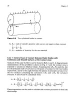
Figure
2.6
Two cylindrical bodies in contact.
RI, R2
=
radii
of
cylinders (positive when convex and negative when concave)
111
E, El
+g
-=-
El,
E2
=
modulus
of
elasticity for the two materials
Case
7:
General Case
of
Contact Between Elastic Bodies with
Continuous and Smooth Surfaces at the Contact Zone
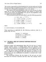
Analysis
of
this case by Hertz can be found in Refs
1

and
2.
A
diagrammatic
representation of this problem is shown in Fig.
2.7
and the contact area is
expected to assume an ellipitcal shape. Assuming that
(RI,
R;)
and
(R2,
R;)
are the principal radii
of
curvature at the point of contact for the two bodies
respectively, and
$
is the angle between the planes of principle curvature for
the two surfaces containing the curvatures
l/R1
and
l/R2,
the curvature
consants
A
and
B
can be calculated from:
These expressions can be used to calculate the contact parameter

P
from the
relations hip:
The
Contact
Between
Smooth Surfaces
31
Figure
2.7
General case
of
contact.
B-A
cos0
=
-
A+B
The semi-axes
of
the elliptical area are:
where
m,
n
=
functions
of
the parameter
8
as

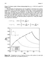
given in Fig.
2.8
P
=
total load
1
-
U:
1
-
u2
nEl
nE2
kl
=-
k2
=
-
ul,
u2
=
Poisson’s ratios for the two
materials
El,
E2
=
corresponding modulii
of
elasticity
Case

8:
Beams on Elastic Foundation
The general equation describing the elastic curve
of
the beam is:
32
Chapter
2
8
degrees
Figure
2.8
Elliptical contact coefficients.
where
k
=
foundation stiffness per unit length
E
=
modulus of elasticity
of
beam material
1
=
moment
of
inertia
of
the beam
With the notation:

the general sohtion for beam deflection can be represented by:
where
A,
B,
C
and
D
are integration constants which must be determined
from boundary conditions.
For relatively short beams with length smaller than
(0.6/8),
the beam
can be considered rigid because the deflection from bending is negligible
compared to the deflection of the foundation. In this case the deflection
will
be
constant and is:
P
s=-
kL
and the maximum bending moment
=
PL/4.
The Contact Between Smooth Surfaces
33
For relatively long beams with length greater than
(5//?)
the deflection
will have a wave form with gradually diminishing amplitudes. The general
solution can be found in texts on advanced strength of materials.

Table
2.2
lists expressions for deflection
y,
slope
8,
bending moment
A4
and shearing force
V
for long beams loaded at the center.
Case
9:
Pressure Distribution Between Rectangular Elastic Bars in
Contact
The determination
of
the pressure distribution between two bars subjected
to concentrated transverse loads on their free boundaries is a common
problem in the design of mechanical assemblies. This section presents an
approximate solution with an empirical linear model for the local surface
contact deformation. The solution is based on an analytical and a photo-
elastic study
[18].
A
diagrammatic representation
of
this problem is shown
Table
2.2

Beam
on
Flexible
Supports
Condition Governing equations"
34
Chapter
2
in Fig. 2.9a. The problem
is
approximately treated as two beams on an
elastic foundation, as shown in Fig. 2.9b. The equations describing the
system are:
where
qX
=
load intensity distribution at the interface (lb/in.)
ZI
,
Z2
=
moments of inertia
of
beam cross-sections
El,
E2
=
modulii of elasticity
zl,
z2

=
local surface deformations
yI,y2
=
beam deflections
kl, k2
=
empirical linear contact stiffness
for
the
two
bars respectively
calculated as:
Et
Et
k2
=-
0.544
kl
=-
0.544
P
Figure
2.9a
Two
rectangular bars in contact.
The Contact Between Smooth Surfaces
35
YI
A

1
1
I I1
I
I
I
11'
kl
I
I
I
t
Y2
Figure
2.9b
Simplified model
for
two
beams in contact.
The criterion for contact requires, in the absence of initial separations, the
total elastic deflection to be equal to the rigid body approach at all points of
contact, therefore:
where
a
is the rigid body approach defining the compliance of the entire
joint between the points where the loads are applied:
The continuity of force at the interface yields:
Equations (2.1)-(2.4) are a system of four equations in four unknowns. This
system is now reduced to a single differential equation as follows. Adding
Eqs

(2.1) and (2.2) gives:
36
Chapter
2
Substituting Eq.
(2.4)
into Eq.
(2.5)
yields:
The combination of Eqs.
(2.3)
and
(2.4)
gives:
Substituting Eq.
(2.7)
into Eq.
(2.6)
yields the governing differential
equation:
where
Kc,
is an effective stiffness:
With the following notation:
Eq. (2.10) may now be rewritten as:
d"
-
+
4$"
=

4$a
d,r4
(2.10)
(2.1
I)
The following are the boundary conditions which the solution of
(2.1
I)
must
satisfy, provided
L
2
C,
where
L
is
half the length of the pressure zone:
The beam deflections are zero at the center location.
The slope is zero at the center.
The summation
of
the interface pressure equals the applied load.
The pressure at the end of the pressure zone is zero.
The moment at the end of the pressure zone
is
zero.
The shear force at the end of the pressure zone is zero.
The six unknowns to be determined by the above boundary conditions are
the four arbitrary constants of the complementary solution, the rigid body
approach

a,
and the effective half-length of contact
C.
The four constants
The
Contact Between Smooth Surfaces
37
and the rigid body approach are determined as a function of the parameter
R
=
/3t.
A plot of the rigid body approach versus
A
is
shown in Fig. 2.10. At
A
=
n/2, the slope of the curve is zero. For values of
R
greater than n/2, the
values of
z1
and
z2
become negative, which is not permitted. The maximum
permitted values of
il
is then n/2 and the effective half-length
of
contact

is
t
=
n/(2/3).
If
n/(2p)
is greater than
L,
the effective length is then
2L.
The expression for the load intensity at the interface is:
cosh
,!?.U
cos
@U
1
PB
(cosh
2A
+
cos
2E.
+
2)
2
sinh
2A
+
sin
21

q=
k1z1
=-
sinh
/!?x
sin
/!?.U
[
(cosh
2i-
COS
2A)
-
(sinh
2;1+
sin
2A)
-
sinh
Bx
cos
Px
+
cosh
Bx
sin
Bx
where
(2.12)
A

=
ge
q
=
the load intensity (lb/in.)
x
=
restricted to
be
0
5
x
5
e
The normalized load intensity versus position is shown in Fig. 2.1
1
for
ge
=
n/2.
This figure represents a generalized dimensionless pressure
distribution for cases where
t
<<
L.
4.0
a
%
3
3.0

U
e
s
a
4
2.0
v)
v)
0
c
0
-

v)
;
1.0
.CI
n
0
.4
.8
1.2
1.6
d2
Figure
2.10
Dimensionless approach
of
the two beams versus the parameter
ge.

38
Chapter
2
Figure
2.1
1
Normalized load intensity over contact region.
The assumption of a constant contact stiffness can be considered ade-
quate as long as the theoretical contact length is far from the ends of the
beams. For cases where
t
approaches
L,
it is expected that the compliance as
well as the stress distribution would be influenced by the free boundary. As a
result, it is expected that the actual pressure distribution would deviate from
the theoretical distribution based
on
constant contact stiffness. A proposed
model for treating such conditions is given in the following. The approx-
imate model gives a relatively simple general method for determining the
contact pressure distributions between beams of different depths which is in
general agreement with experimental pho
t
oelas
t
ic investigations.
In the model the contact half-length
t
is

calculated from the geometry of
the beam according to the formula:
When
t
<<
L,
the true half-length of contact is equal to
t
and the corre-
sponding pressure
is
directly calculated from Eq. (2.12) or directly evaluated
from the dimensionless plot of Fig. 2.11.
As
t
approaches
L,
the effect
of
the free boundary comes into play and
the constant stiffness model can no longer
be
justified. An empirical method
The Contact Between Smooth Surfaces
39
to deal with the boundary effect for such cases is explained in the following.
The method can be extended for the cases where
C
2
L.

Because of the increase in compliance at the boundaries of a finite beam
as the stressed zone approaches it, a fictitious theoretical contact length
l’(e’
>
e)
can be assumed to describe a hypothetical contact condition for
equivalent beams with
L‘
>>
e
(according to the empirical relationship given
in Fig. 2.12. The pressure distribution for this hypothetical contact condi-
tion
is
then calculated. Because the actual half-length of the beam is
L,
it
would
be
expected that the pressure between
e’
and
L
would have to be
carried over the actual length
L
for equilibrium. The redistribution
of
the
pressure outside the physical boundaries of the beam is assumed to follow a

mirror image, as shown in Fig.
2.13.
The superposition of this reflected pressure on the pressure within the
boundaries of the beam gives the total pressure distribution.
The general procedure cam be summarized as follows:
1.
2.
3.
Calculate
/3
from geometry and the material of the contacting bars
according to Eq.
(2.10).
Calculate
l
from the equation
t
=
n/(2/3).
Using
e
and
L,
find
f?’
from Fig.
2.12.
Notice that for
e
<<

L,
e’
=
e.
1.8
1.6
h
$
1.4
3
1.2
1
.o
0
.4
.8
1.2 1.6
2.0
(L
f
4
Figure
2.1
2
Empirical relationship for determining
t!
’.
40
Chapter
2

Boundary
i-
Figure
2.13
The
“mirror
image” procedure.
4.
5.
6.
Evaluate the pressure distribution over
l’
from the normalized
graph, Fig.
2.1
1.
For
l
<<
L,
the pressure distribution as calculated in step
4
is
the
true contact pressure.
When
t’
is greater than
L,
the distribution calculated by step

4
is
modified by reflection
(as
a mirror image
of
the pressure outside
the physical boundaries defined by the length
t).
2.3
A MATHEMATICAL PROGRAMMING METHOD FOR
ANALYSIS AND
DESIGN
OF
ELASTIC BODIES
IN
CONTACT
The general contact problem can be divided into two categories:
Situations where the interest is the evaluation of the contact area, the
pressure distribution, and rigid body approach when the system
configuration, materials and applied loads are known;
Systems which are to be designed with appropriate surface geometry for
the objective of obtaining the best possible distribution of pressure
over the contact region.
In this section a general formulation is discussed for treating this class
of
problems using a modified linear programming approach.
A
simplex-type
algorithm is utilized for the solution

of
both the analysis and design situa-
tions.
A
detailed treatment
of
this problem can be found in Refs
18
and
19.
The Contact Between Smooth
Surfaces
41
2.3.1
The Formulation
of
the Contact Problem
The contact problems which are analyzed here are restricted to normal
surface loading conditions. Discrete forces are used to represent distributed
pressures over finite areas. The following assumptions are made:
1.
The deformations are small.
2.
3.
The two bodies obey the laws
of
linear elasticity.
The surfaces are smooth and have continuous first derivatives.
Problem formulation and geometric approximations can therefore be made
within the limits

of
elasticity theory.
2.3.2
Condition
of
Geometric Compatibility
At any point
k
in the proposed zone of contact (Fig.
2.14),
the sum
of
the
elastic deformations and any initial separations must be greater than or
equal to the rigid body approach. This condition is represented as:
where
&k
=
initial separation at point
k
a
=
rigid body approach
\l’k(l),
kt’k(2)
=
elastic deformations
of
the two bodies respectively at point
k

Figure
2.14
Zone of contact.
42
Chapter
2
2.3.3
Condition
of
Equilibrium
The sum of all the forces
F’
acting at the discrete points
(k
=
1,
.
.
.
,
N
where
N
is the number of candidate points for contact) must balance the applied
load
(P)
normal to the surface. The equilibrium condition can therefore be
written as:
(2.14)
2.3.4

The Criterion
for
Contact
At any point
k,
the left-hand side of the inequality constraint in Eq.
(2.13)
may be strictly positive or identically zero. Defining a slack variable
Yk
representing a final separation, the contact problem can
be
formulated as
follows.
Find a solution
(F,
a,
Y)
which satisfies the following constraints:
-SF+cre+IY=e
eTF
=
P
(2.15)
Either
where
skj
=
akj,(l)
-k
akj(2)

akj(l), akj(2)
=
influence coefticients for the deflection of the two bodies respectively
skj
=
N
x
N
matrix of influence coefticients
F
=
N
x
1
vector
of
forces
Y
=
N
x
1
vector
of
slack variables (or final separation)
e
=
N
x
1

vector
of
1’s
E
=
N
x
1
vector
of
initial separations
(Y
=
rigid body approach, a scalar
The
Contact
Between Smooth
Suflaces
43
2.4
A
GENERAL METHOD
OF
SOLUTION
BY
A
SIMPLEX-TYPE
ALGORITHM
The problem as formulated in Eq.
(2.15)

can be solved using a modification
of the simplex algorithm used in linear programming. The changes required
for the modification are minor and are similar to those given by Wolfe
[S].
When Eq. (2.15) is represented in a tableau form in Table 2.3, the condition
for the solution can be stated as:
Find the set of column vectors corresponding to
(F,
a,
Y)
subject to the
conditions, either
Fk
=
0
or
Yk
=
0,
such that the right-hand side is
a nonnegative linear combination of these column vectors. These
column vectors are called a basis.
For a problem with
N
discrete points, the number of possible combinations
of these column vectors taken
(N
+
1)
at a time is:

Because of the very large number of combinations,
an
efficient method is
required for finding the unique, feasible solution. The following algorithm
proved to be effective for the problem under investigation.
The original problem as formulated in Eq. (2.15) can be rewritten
as:
N+l
Minimize
XZ,
j=
I
such that
-SF
+
ae
+
IY
+
Iz
=
E
eTF
+
ZN+I
=
P
Table
2.3
Representation

of
Eq.
(2.15)
(2.16)
Fl
F2

FN
YI
y2

YN
1
=
62
+1
+I
+
+1
=P
44
Chapter 2
Subject to the conditions that
Either
where
Zj
=
artificial variables which are required to
be
nonnegative

(j
=
1,
. .
.
,
N
+
1)
2
=
an
N
x
1
vector
of
artificial variables
with
components
Z,,
.
. .
,
ZN
-
The above problem can be classified as a linear programming problem
[
131 if
it

were not for the condition that either
Fk
=
0
or
Yk
=
0.
The simplex
algorithm for linear programming can, however, be utilized to solve by
making a modification of the entry rules.
The conditions of Eq. (2.15) require some restrictions on the entering
variables. Suppose the entering variable
is
chosen as
F,.
A
check must be
made to see if the
Y,
is not in the basis,
F,
is free
to
enter the basis.
The actual replacement of variables is accomplished by an operation
called pivoting. This pivot operation consists of
N
+
1

elementary opera-
tions which replace a system by an equivalent system in which a specified
variable has a coefficient of unity in one equation and zero elsewhere
[
131.
A
flow diagram of the modified simplex algorithm is shown in Fig. 2.15.
Computational experience has shown the simplex-type algorithm to
converge
to
the unique feasible point in at most (3/2)(N+
1)
cycles, the
majrity of cases converge in
N
+
1
cycles.
The simplex-type algorithm for the solution of the contact problem
requires less computer storage space when compared to available solution
algorithms such as Rosen's gradient projection method
[14]
or the Frank-
Wolfe algorithm
[
151. Only minor modifications of the well-known simplex
algorithm are required. This algorithm is also readily adaptable
to
the
design problem which is discussed later in this section.

EXAMPLE
1.
The classical problem of two spheres in contact is consid-
ered as an example. In this case the influence coefficient matrix
S
in
Eq.
(2.15)
is
calculated according to a Boussinesq model as discussed earlier
in this chapter:
The Contact Between Smooth Surfaces
I
I
r
45
,
No
P
Start
with
standard equations
N+l
j-I
1
=
c
zj
t
Define

J=(jllIjIZN+I}
*
,
Make canonical
relative
to
the
artificial variables
r-
and
2'
Choose
s
by
d,
=
mindj
jd
Test
min
4)
is
d,
2
O?
I
Chooserby
I
Basic feasible
solution

If
s
corresponds to
Ff
is
V,
in
the Basis?
If
scorresponds to
Y,
Is
6)
>
O?
I
-
A
Yes
Would
Fr
replace
5.
or
V,
replace
4.
Remove
s
from

J
STOP
No
feasible
solution
No
Replace
the
r'*
basic variable
by
x,
by pivoting on
the term
a,x,
Define
4
J
=
(Jll
I
j
I
2N
+
1)
-
Figure
2.1
5

Flow
diagram for the simplex-type algorithm.
where
U
=
Poisson's ratio
dk,
=
distance
from
point
k
to pointj in the contact zone
Figure 2.16 shows a comparison between the classical Hertzian pressure
distribution and that obtained
by
the described technique. The spheres con-
sidered are steel with radii of
1
in.
and
loin., respectively and the applied
load is 1001b. The algorithm solution gave a value of 0.000281
in.
for the
rigid body approach which compares favorably with 0.000283 in. for the
classical Hertz solution.
46
Chapter
2

180,000
-
12
-
h
.r(
v
v)
g
120,000
&
2
60,000
-
3
-
0
Classical Theory
-
Computer
Based
Model
-
-
with
11
Points
Across
the
Diameter

m
U
c,
0
.0150
.0100
.0050
0
.0050
.0100
.0150
Radial Distance
from
the Applied
Load
(in)
Figure
2.1
6
Pressure distribution between two spheres.
2.5
THE DESIGN PROCEDURE FOR UNIFORM LOAD
DISTRIBUTION
The design system discussed in this section automatically produces initial
separations which produce the best possible distribution of load based on a
selected function for surface modification (initial separation).
A
second-
order curve is selected for the initial separation since it can be readily
generated. The equation for such curve is given by:

y
=
ox2
+
bx+
c
(2.17)
where
y
=
initial separation profile and is required to be
2
0
.Y
=
axial position along the face
The correction profile can be attained by modifying one or both of the
contacting surfaces. The objective of the design system
is
to evaluate the
constants
(a,
b,
c)
for
the optimal corrections corresponding to the distribu-
tion giving the minimum possible value for the maximum load intensity.
In the formulation of the design system the compatibility condition
given in
Eq.

(2.15)
is
used with
E
being replaced by
Eq.
(2.17). Accordingly:
-SF
+
aye
+
IY
-
aX2
-
bX
-
c
=
0
(2.18)
The Contact Between Smooth Surfaces
47
where
-2
X
=
N
x
1

vector whose kth element is
xi
X
=
N
x
1
vector whose kth element
is
xk
xk
=
position
of
the kth point
-
The condition of equilibrium and the criterion for contact are the same as in
Eqs (2.14) and (2.15).
The initial separations are required to be nonnegative, therefore:
ay2
+by+
c
2
0
where
a
governs the sign of the second derivative.
If we define Ak as the length of the line segment at the kth point, the
average load intensity over that segment is Fk/Ak. The value
of

pmax
must be
greater than the average load intensities at all the candidate points. This
constraint is written as follows:
where
D
is a diagonal matrix whose kth element is l/Ak.
The design system is now stated in a concise form as:
Minimize
pmax
such that
e'F=P
F,
Y,
a,
c
2
0
Subject to the condition that either
Yk
=
0
or
Fk
=
0
(2.19)
It should be noted that an upper bound must be given to
c
to

keep the values
of
c
and
a
finite in
Eq.
(2.19).
The algorithm for solving the design problem (Fig.
2.17)
is divided into
two parts. The first part finds
a
feasible solution for the load distribution
48
Chapter
2
while the initial separations are constrained to be zero. The second part
minimizes the maximum load intensity using the parameters
(a,
b,
c)
as
design variables. The simplex-type algorithm is used in both parts.
The minimization of the maximum load intensity
is
a nonlinear pro-
gramming problem, the objective function is linear but the constraints are
nonlinear
[

171. Since all the constraints are linear except for the criterion for
contact, the basic simplex algorithm can again be used with the modified
entry rules as discussed previously.
EXAMPLE
2. The case of a steel beam on an elastic foundation is con-
sidered here as an illustration of the design system. It is required in this
case to calculate the necessary initial separations which produce, as closely
as possible, a uniform pressure. Given in this example are:
L,
t,
and
d
=
length, width, and depth of beam
=
8.9
in.,
1.0
in., and
4.0
in., respectively
k
=
foundation modulus
=
10’
lb/in./in.
The results from the solution algorithm with a quadratic modification are
given in Figs 2.18 and 2.19 and the pressure distribution without initial
separation is shown in Fig.

2.18
for comparison. The initial separation as
calculated from the analysis program for a uniform pressure distribution is
also shown in Fig. 2.19. It can be seen that the quadratic modification,
although it does not provide an exactly uniform pressure distribution, repre-
sents the best practical initial separation for the stated objective.
An approximation for evaluation
of
the surface modification can be
obtained by assuming a uniform load distribution, computing the necessary
initial separations and then fitting these data to a curve with the stated form
of
surface modification. In the process of curve fitting, the main objective is
to approximate the computed initial separations without regard to the
resulting load distribution.
The same approach can be readily applied
to
the surface modification of
bolted joints
to
produce uniform pressure in the joint and consequently
minimize the tendency for leakage or fretting depending on the application.
EXAMPLE
3.
In this example, the same approach is applied for deter-
mining the initial separation necessary to produce uniform pressure at the
interface between multiple-layered beams. The case considered for illustra-
tion is shown in Fig.
2.20
where three cantilever beams are subjected to

The Contact Between Smooth
Surfaces
49
Sm
with
rhc
Standard
Equations
(5.18)
Add
the artificial
variables
Z1
.Z2,
,
Z,,,
Add
objective function
z,
=
z
zj
j=1
Make canonical relative
to
the artificial variables,
Define
J=
the
set

of
all
variabks
exap
a.
6.
E
1
,
.
Jo
1
I
Ifs
cornponds
to
F,
is
Y,
in
the
basis?
or
Ifs
cormponds
to
Y,
is
F,
in

thc
basis?
-
Yes
r
No
1
I
Choosesby
I
min
Choose
s
by
d;
=-
Would
F,
J“‘
dJ
i”’
Ji
3
nplm
r,
OT
Test
min
P-
d;

-
min
+
r,
replace
F,?
Is
Ds2
O?
No
YC.5
Is
d.;
2
O?
Test
min
Z,
A/
A’
Yes
V
\L
vv
STOP
Remove
s
Best
Basic
fivrnJ

Replace
the
r*
Feasible
STOP
basic variable by
Solution
No
xs
by pivoting on
the term
ursxs
Phase
I
Phase
I1
Fusible
Is
2,
>
O?
Solution
No
*
allvllriablcs
-
all vahblu
except
I
I

I
stan
Phase
I1
Design
Phasc
Use
the
pmPx
row
Basic
Feasible
Solution
-_


Figure
2.1
7
Flow
diagram for
the
design algorithm.
50
Chapter
2
Figure
2.1
8
Pressure distribution of beam on elastic foundation.

2.0
-
Optimum Quadratic Correction
0
.LI
c)
(d
'3
C
n
.d
Pressure
I
i
i
I
0
1
2
3
4
5
Distance
From
Center
of
Beam
(in.)
Fiaure
2.1

9
Initial separation for uniform pressure distribution and optimal
quadratic correction.
The Contact Between Smooth
Surfaces
51
P
Figure
2.20
Multiple cantilever
beams.
an end load. The applied load
P
is assumed to be 60001b, the length
of
the beam is 12in. and width is
1
in. and the thicknesses are 5in., 2in. and
5in., respectively. The beams are made of steel with modulus of elasticity
equal to
30
x
106psi. The interface areas are divided into 24 segments and
the force on each segment is found to be
70.621b
for both interfaces
which is equivalent to 141.24 psi. The calculated initial separations are
given in Fig. 2.21.
Interface
1

(F
=
70.62
Ib
at
each
point)
o
0
0
0
0
0
0
no
0
-0
0
"OOU
0
0
Q
tl
Interface
2
(F=
70.62
Ib
at
each

point)
-0-
-
2
4
6
8
10
12
Hl=5,
HZzO.1,
H3=5
Distance
From
the
Fixed
End (in.)
Figure
2.21
Initial separations.
52
Chapter
2
103
102
10
1
0.1
H,=5
in.

-
-
-
-
h
K
2
10-2
10-3
-
t,
-
104
10-5
10-6
1
I
I
I11111
I
I
I111111
1
I
11
Ill11
I I
I1
11111
1

I
I
I
LLU
EXAMPLE
4.
In this case a steel cantilever beam with length
12in.,
width
I
in. and thickness 3in. is subjected to an end load of 60001b. The
beam is supported
by
another steel cantilever beam with the same length
and width and different thickness
H2
as shown in Fig. 2.22. The same
algorithm is used with
24
segments at the interface to determine the maxi-
mum attainable uniform pressure at the interface and the corresponding
initial separation
Smax
at the free end for different values
of
the thickness
Hz.
The results are given in Fig. 2.23 and show that
Smax
will reach an

asymptotic limit when
H2
is either very large or very small. The uniform
load on each segment
F,,,
is shown to reach
a
limit value when
H2
is
very large.
.01
.008
.OM
2
2
."
W
K
.004
-
.002
0
FN
FI,
F2,

X-
Figure
2.22

Discrete forces.
.ration.
The Contact Between Smooth
Surfaces
53
Numerous illustrative examples for simulated bolted joints, multiple
A
list of some of the publications dealing with different aspects
of
the
layer beams and elastic solids with finite dimensions are given in Ref.
20.
contact problem is given in Refs
21-39.
REFERENCES
1.
2.
3.
4.
5.
6.
7.
8.
9.
10.
11.
12.
13.
14.
15.

16.
17.
Timoshenko, S.P., Theory of Elasticity, McGraw Hill Book Company, New
York,
1951.
Love, A. E.
H.,
A Treatise on the Mathematical Theory of Elasticity, Dover,
New York,
1944.
Timoshenko,
S.
P., Strength of Materials, Part 11, D. Van Nostrand, New
York,
1950.
Galin, L. A., Contact Problems in the Theory of Elasticity, Translation by
H.
Moss, North Carolina State College,
1961.
Keer, L. M., “The Contact Stress Problem for an Elastic Sphere Indenting an
Elastic Layer,” Trans. ASME, Journal
of
Applied Mechanics,
1964,
Vol.
86,
Tu, Y
.,
“A Numerical Solution for an Axially Symmetric Contact Problem,”
Trans. ASME, Journal of Applied Mechanics,

1967,
Vol.
34,
pp.
283.
Tsai, N., and Westmann, R. A., “Beam on Tensionless Foundation,” Proc.
ASCE, J. Struct. Div., April
1966,
Vol.
93,
pp.
1-12.
Wolfe, P., “The Simplex Method for Quadratic Programming,” Econometrica,
Dorn, W.
S.,
“Self-Dual Quadratic Programs,” SIAM
J.
Appl. Math.,
1961,
Cottle, R. W., “Nonlinear Programs with Positively Bounded Jacobians,”
JSIAM Appl. Math.,
1966,
Vol.
14(1),
pp.
147-158.
Kortanek, K., and Jeroslow,
R.,
“A
Note on Some Classical Methods in

Constrained Optimization
and
Positively Bounded Jacobians,” Operat
.
Res.,
1967,
Vol.
15(5),
pp.
964-969.
Cottle, R. W., “Comments on the Note by Kortanek and Jeroslow,” Operat.
Res.,
1967,
Vol.
15(5),
pp.
964-969.
Dantzig,
G.
W., Linear Programming and Extensions, Princeton University
Press, Princeton, NJ,
1963.
Rosen,
J.
B., “The Gradient Projection Method for Non-Linear
Programming,” SIAM J. Appl. Math.,
1960,
Vol.
8,
pp.

181-217; 1961,
Vol.
9,
pp.
514-553.
Frank, M., and Wolfe, P., “An Algorithm for Quadratic Programming,” Naval
Research Logist.
Q.,
March-June
1956,
Vol.
3(1
&
2),
pp.
95-1
10.
Kerr, A.
D.,
“Elastic and Viscoelastic Foundation Models,” Trans. ASME,
J. Appl. Mech.,
1964,
Vol.
86,
pp.
491-498.
Mangasarian,
0.
L., Nonlinear Programming, McGraw Hill Book Company,
New York, NY,

1969.
pp.
143-145.
1959,
Vol.
27,
pp.
328-398.
Vol.
9,
pp.
51-54.
54
Chapter
2
18.
19.
20.
21.
22.
23.
24.
25.
26.
27.
28.
29.
30.
31.
32.

33.
34.
35.
Conry,
T.
F., “The
Use
of Mathematical Programming in Design for Uniform
Load Distribution in Nonlinear Elastic Systems,” Ph.D. Thesis, The University
of Wisconsin, 1970.
Conry, T. F., and Seireg, A., “A Mathematical Programming Method for
Design of Elastic Bodies in Contact,,’ Trans. ASME, J. Appl. Mech., 1971,
Ni, Yen-Yih, “Analysis
of
Pressure Distribution Between Elastic Bodies with
Discrete Geometry,” M.Sc. Thesis, University of Florida, Gainesville, 1993.
Johnson,
K.
L., Contact Mechanics, Cambridge University Press, New York,
NY, 1985.
Ahmadi, N., Keer,
L.
M., and Mura, T., “Non-Hertzian Contact Stress
Analysis
-
Normal and Sliding Contact,” Int. J. Solids Struct., 1983, Vol. 19,
Alblas, J. B., and Kuipers, M., “On the Two-Dimensional Problem of a
Cylindrical Stamp Pressed into a Thin Elastic Layer,” Acta Mech., 1970,
Vol. 9, p. 292.
Aleksandrov, V. M., “Asymptotic Methods in Contact Problems,’’ PMM,

1968, Vol. 32,
pp.
691.
Andersson, T., Fredriksson, B., and Persson, B. G. A., “The Boundary
Element Method Applied
to
2-Dimensional Contact Problems,” New
Developments in Boundary Element Methods. CML Publishers,
Southampton, England, 1980.
Barovich,
D.,
Kingsley,
S.
C.,
and
Ku,
T.
C.,
“Stresses on a Thin Strip or Slab
with Different Elastic Properties from that of the Substrate,” Int. J. Eng. Sci.,
1964, Vol. 2, p. 253.
Beale,
E.
M. L., “On Quadratic Programming,’, Naval Res. Logist. Q., 1959,
Vol. 6, p. 74.
Bentall, R. H., and Johnson,
K.
L.,
“An Elastic Strip in Plane Rolling
Contact,,’ Int.

J.
Mech. Sci., 1968, Vol. 10, p. 637.
Calladine, C.
R.,
and Greenwood,
J.
A., “Line and Point Loads on a Non-
Homogeneous Incompressible Elastic Half-Space,” Quarterly Journal
of
Mechanics and Applied Mathematics, 1978,
Vol.
3
1, p. 507.
Comniou, M., “Stress Singularities at a Sharp Edge in Contact Problems with
Friction,” ZAMP, 1976, Vol. 27, p. 493.
Dundurs, J., Properties
of
Elastic Bodies in Contact, Mechanics
of
Contact
between Deformable Bodies, University Press, Delft, Netherlands, 1975.
Greenwood, J. A., and Johnson,
K.
L., “The Mechanics of Adhesion
of
Viscoelastic Solids,” Philosphical Magazine, 1981, Vol. 43, p. 697.
Matthewson, M. J., “Axi-Symmetric Contact on Thin Compliant Coatings,”
Journal of Mechanics and Physics of Solids, 1981, Vol. 29, p. 89.
Maugis, D., and Barquins, M., “Fracture Mechanics and the Adherence
of

Viscoelastic Bodies,’, Journal of Physics
D
(Applied Physics), 1978, Vol.
1
1.
Meijers, P., “The Contact Problems
of
a Rigid Cylinder on an Elastic Layer,”
Applied Sciences Research, 1968, Vol. 18,
p.
353.
Vol. 38, pp. 387-392.
p. 357.