Friction and Lubrication in Mechanical Design Episode 1 Part 4 docx

The
Contact
Between Smooth
Surfaces
55
36.
37.
Mossakovski,
V.
I.,
“Compression of Elastic Bodies Under Conditions of
Adhesion,” PMM,
1963,
Vol.
27,
p.
418.
Pao,
Y.
C.,
Wu,
T.
S.
and Chiu,
Y.
P., “Bounds on the Maximum Contact
Stress of an Indented Layer,” Trans. ASME Series E, Journal of Applied
Mechanics,
1971,
Vol.
38,

p.
608.
Sneddon,
I.
N.,
“Boussinesq’s Problem for a Rigid Cone,” Proc. Cambridge
Philosphical Society,
1948,
Vol.
44,
p.
492.
Vorovich,
1.
I.,
and Ustinov,
I.
A.,
“Pressure of a Die on an Elastic Layer of
Finite Thickness,” Applied Mathematics and Mechanics,
1959,
Vol.
23,
p.
637.
38.
39.
3
Traction Distribution and Microslip in
Frictional Contacts

Between
Smooth
Elastic Bodies
3.1
INTRODUCTION
Frictional joints attained by bolting, riveting, press fitting, etc., are widely
used for fastening structural elements. This chapter presents design formulae
and methods for predicting the distribution
of
frictional forces and micro-
slip over continuous or discrete contact areas between elastic bodies sub-
jected
to
any combination
of
applied tangential forces and moments. The
potential areas for fretting due to fluctuation of load without gross slip are
discussed.
The analysis of the contact between elastic bodies has long been of
considerable interest in the design of mechanical systems. The evaluation
of
the stress distribution in the contact region and the localized microslip,
which exists before the applied tangential force exceeds the frictional resis-
tance, are important Factors in determining the safe operation of many
structural systems.
Hertz
[l]
established the theory for elastic bodies in contact under
normal loads. In his theory, the contact area, normal stress distribution
and rigid body approach in the direction

of
the common normal can be
found under the assumption that the dimensions of the contacting bodies
are significantly larger than the contact areas.
Various extensions of Hertz theory can be found in the literature
[2-151,
and the previous chapter gives an overview of procedures for evaluating the
area
of
contact and the pressure distribution between elastic bodies
of
arbi-
trary smooth surface geometry resulting from the application
of
loading.
56
Traction Distribution and Microslip in Frictional Contacts
57
An important class of contact problems is that of two elastic bodies
which are subjected to a combination of normal and tangential forces.
The evaluations of the traction distribution and the localized microslip
on the contact area due to tangential loads are important factors in deter-
mining the safe operation of many structural systems. Several contributions
are available in the literature which deal with the analytical aspects of this
problem
[16-191.
The contact areas considered in all these studies are, how-
ever, limited to either a circle or an ellipse, and a brief summary
of
the

results of both cases is given in the following section.
This chapter also presents algorithmic solutions which can
be
utilized
for the analysis of the general case of frictional contacts. Three types of
interface loads are to be expected: tangential forces, twisting moments, and
different combinations of them. When the loads are lower than those neces-
sary to cause gross slip, the microslip corresponding to these loads may
cause fretting and surface cracks. The prediction of the areas of microslip
and the energy generated in the process are therefore of considerable interest
to the designer of frictional joints.
3.2
TRACTION DISTRIBUTION, COMPLIANCE, AND ENERGY
DISSIPATION
IN
HERTZIAN CONTACTS
3.2.1
Circular Contacts
As
shown in Fig.
3.1,
when two spherical bodies are loaded along the
common normal by a force
P,
they will come into contact over an area
with radius
a.
When the system is then subjected to a tangential force
T
<

fP,
Mindlin’s theory
[
161 for circular contacts defines the traction dis-
tribution over the contact area and can be summarized as follows:
113
a*
=
a(
I
-;)
F,,
=
0
over the entire surface
58
Chapter
3
lp
1
-T
Figure
3.1
The contact of spherical bodies.
where
F,,
l$
=
traction stress components at any radius
p

a
=
radius
of
a
circular contact area
p
=
(x2
+y2)'I2
=
polar coordinate
of
any point within the contact area
T
=
tangential force
P
=
normal load
f
=
coefficient of friction
G
=
shear modulus of the material
U
=
Poisson's ratio
a*

=
radius defining the boundary between the slip and no-slip regions
Figure
3.2
illustrates the traction distribution as defined
by
Eqs
(3.1)
and
(3.2).
It
can be seen that
a*
=
a
for
T
=
0
and no microslip occurs;
U*
=
0
for
T
=
fP
and the entire contact area is in a state
of
microslip and impending

gross
slip.
Traction Distribution and Microslip in Frictional Contacts
59
I
t
1
a*
fqo
-
a
6-
PQO
i
I
I
b
a* a
T
P
Figure
3.2
Traction distribution
for
circular contact
(90
=maximum contact
pressure
=
3P/(2rra2)).

The deflection
S
(rigid body tangential movement) due to the any load
T
>fP
can be calculated
from:
Consequently, at the condition
of
impending gross slip,
T
=fP:
(3.4)
The traction distribution and compliance for a tangential load fluctuating
between
fT*
(where
T*
cfP)
can be calculated as follows (see Figs
3.3
and
3.4):
60
Chapter
3
P
Figure
3.3
Traction distribution for decreasing tangential load

T
-=
T*.
h*
=
inner radius of slip region
U*
=
inner radius
of
slip region at the peak tangential load
T*
I
/z
F,
=
-jiqO[
1
-
(!)‘I
F,
=
+,,[
1
-
(5)2]”2+2j4!3
[
1
-
02]

U*
5
p
5
b*
F,
=
-JqO
[
1
-
(92]1f2
-
+2jq0
.
(:)[
-
1
-
(;)*]”’-fq0@[l
-
h*
5
p
5
a
2
10
-
(5)

]
P
<
a*
Traction Distribution and Microslip
in
Frictional Contacts
61
Figure
3.4
Hysteresis
loop.
where
3P
yo
=
maximum contact pressure
=
-
2na2
The deflection can
be
calculated
from:
Sd
=
deflection
for
decreasing tangential load
-

3(2
-
u)fP
[
2
(
I
T*
-
T)2'3
-
(
I
7'7')2'3]
-
16Ga
2fP
for
T
decreasing from
T*
to
-T*;
Sj
=
-6&T)
-_
-
3(2 -8)fP[
2

(
1
T*
+
q"
(
T*)2'3
-
-
l-fp
16Ga
2fP
for
T
increasing from
-T*
to
T*.
62
Chapter
3
The frictional energy generated per cycle due to the load fluctuation can
therefore be calculated from the area of the hysteresis loop as:
M’
=
work done as a
T’
=
I
(Sd

-
&)dT
-
T’
result of the microslip per cycle
(3.5)
(
T*)5’3

ST*
[
1-
(
I
T*)2’3]]
-
I-fp
6fP fP
3.2.2
Elliptical Contacts
A
similar theory was developed by Cattaneo [17] for the general case of
Hertzian contacts where the pressure between the two elastic bodies occurs
over an elliptical area. Cattaneo’s results for the traction distribution in this
case can be summarized as follows:
on slip region
F,,
=
0
for the entire surface

where
a,
b
=
major and minor axes of an elliptical contact area
a*,
b*
=
inner major and minor axes of the ellipse defining the boundary between
the slip and no-slip regions
3.3
ALGORITHMIC SOLUTION
FOR
TRACTION DISTRIBUTION
OVER CONTACT
AREA
WITH ARBITRARY GEOMETRY
SUBJECTED TO TANGENTIAL LOADING BELOW
GROSS
SLIP
This section presents a computer-based algorithm for the analysis of the
traction distribution and microslip in the contact areas between elastic
Traction Distribution and Microslip in Frictional Contacts
63
bodies subjected to normal and tangential loads. The algorithm utilizes a
modified linear programming technique similar to that discussed in the
previous chapter. It is applicable to arbitrary geometries, disconnected con-
tact areas, and different elastic properties for the contacting bodies. The
analysis assumes that the contact areas are smooth and the pressure distri-
bution on them for the considered bodies due to the normal load is known

beforehand or can be calculated using the procedures discussed in the
previous chapter.
3.3.1
Problem Formulation
The following nomenclature
will
be used:
x,
y
=
rectangular coordinates of position
U,
v
=
rectangular coordinates
of
displacement in the
x-
and y-directions
respectively
E
=
Young’s modulus
v
=
Poisson’s ratio
G
=
modulus of rigidity
P

=
applied normal force
T
=
applied tangential force
f
=
coefficient of friction
N
=
number of discrete elements in the contact grid
Fk
=
discretized traction force in the direction of the tangential force
uk
=
discretized displacement force in the direction of the tangential
F,.,
F,:
=
rectangular components of traction on a contact area
at any point
k
force at any point
k
force at point
k
point
k
ylk

=
displacement slack variables in the direction of the tangential
yuc
=
force slack variables
in
the direction of the tangential force at
The contact area is first discretized into a finite number of rectangular grid
elements. Discrete forces can be assumed to represent the distributed shear
traction over the finite areas
of
the mesh. Since the two bodies in contact
64
Chapter
3
obey
the laws of linear elasticity, the condition for compatibility of defor-
mation can therefore be stated as follows:
uk
=
p
uk
<
p
in the no-slip region
in
the slip region
where the difference between the rigid body movement
/?
and the elastic

deformation
uk
at any element in the slip region is the amount of slip.
The constraints on the traction values can also be stated as:
Fk
<f’Pk
Fk
=fPk
in
the no-slip region
in
the slip region
(3.7)
where
Fk
=
the discretized traction force in the
x
direction at any point
k
Pk
=
the discretized normal force at any point
k
f’
=
the coefficient of friction
The condition for equilibrium can therefore be expressed as:
Introducing
a

set of nonnegative slack variables
Ylk
and
Y2k,
Eqs
(3.6)
and
(3.7)
can be rewritten as follows:
where
)‘I,
=
0
?‘lk
’
0
where
Y2k
’
0
U,,
=
0
Uk
+
Y,k
=
#?
in
the no-slip region

in the slip region
Fk
4-
Y2k
=
fpk
in
the no-slip region
in
the slip region
(3.9)
(3.10)
Since a point
k
must be either in the no-slip region or in the slip region,
therefore:
Traction Distribution
and
Microslip in Frictional Contacts
65
3.3.2
General Model for Elastic Deformation
Since both bodies are assumed to obey the laws of elasticity, the elastic
deformation
uk
at a point
k
is a linear superposition of the influences of
all the forces
4

acting on a contact area. Accordingly:
(3.12)
j=
1
where
ay
=
the deformation in the x-direction at point k due
to
a unit force at point
j
The discrete contact problem can now be formulated in a form similar to
that given in Chapter
2
as:

-
Find
(F,
Y1,
Yz,
/?)
which satisfies the following constraints:
where
A
=
N
x
N
matrix

of
influence coeficients
I
=
N
x
N
identity matrix
F
=
discretized tangential
force
vector
-

Yl
,
Y2
=
slack variable vectors
-
P
=
discretized normal force vector
e
=
vector of
1’s
The problem can be restated in a
form

suitable for solution
by
a modified
linear program as follows:
2N+1
Minimize
z,
i=
I
66
Chapter
3
dative
to
artificial variables and objective
value
ID
uable
1)
Yes
I
1
No
Choose entering column
s
according to
Brand's
rule
s
=

min
(j
E
[
JSTART,3N
+
l]d, <
0)
I
Is
(D
almost
r<T>-,
Print the feasible
solution
and
stop
solution.
stop
/
Ifsconespondsto
\
asis?
or
Ifs
corresponds
to
No
Y,,
is

Y,
in
the
Would
Y,,
replace
Y,
1"
Would
Y,,
would
Y,
Yes
replace
Y,
Of
No
t
1
START
=
s+l
Replace the rth
basic
variable
by
the 8th variable
with
Jordan
exchange

by
pivoting on
a,,
(a)
FiQure
3.5
(a) Flow chart
for
the analysis algorithm. (b) Initial table.
Traction Disfribution and Microslip in Frictional Contacts
67
where
E
:
a
cost
coefficient
vector
of
length
N
N
c,
=-Car
-2
bl
CO
:
initial
merit

value
(b)
tD
=-fP-T
subject to
AF+I~,
-/?e+IZI
=O
IF++72+IZ2=fF
eTF
+
Z2N+I
=
T
Ylk
=
0
or
Y2k=0
fork=
I,
,
N
Fk>O,
YlkzO,
Y.20,
/?rO
fork=l,
,
N

zi
2
0
for
i=
1,
,
2N+
1
where
-
2,
=
first
N
artificial variable vector
Z2
=
next
N
artificial variable vector
-
22N+1
=
artificial variable for the equilibrium equation
The above problem can be solved
as
a
linear programming problem
[20]

with a
modification
of
the entry rule. Suppose the entering variable is chosen as
Y,,.
A
check must be made to see if the
Ya
corresponding
Y1,
is in the basis and if
the
Y2.$
is not in the basis,
Y1,
is free to enter the basis. If
Yr,
is in the basis, then
it must be in the leaving row,
r,
for
Yl,
to enter the basis. If
Y2.$
is
not in the
leaving row,
r,
Y1,
cannot enter the basis and

a
new entering variable must be
chosen. The same logic can
be
applied when the chosen entering variable is
YZs.
The flow chart for the algorithm utilizing linear programming with
modified entry rule is shown in Fig.
3.5.
68
Chupter
3
It
is
assumed for
the
circular and elliptical contacts that the surface of
contact is very small compared to the radii of curvature of the bodies;
therefore, the solution obtained for semi-infinite bodies subjected to point
loads can be employed. Accordingly, the influence coefficients,
akj,
can be
expressed as follows [21, 221:
If
k
#
j,
then
1
1

-
u2
x;j
u(l
+
U)
Akj
=
-
-
+
nrkj
E
nr;j
E
If
k
=
j,
then
where
3.3.3
Illustrative Examples
EXAMPLE
1:
Circular Hertzian Contact with Similar Materials.
The
first application of the developed algorithm is finding the traction dis-
tribution over the contact area of a steel sphere of
1

in. radius on a steel
half space. The normal load is taken as 21601bf, the tangential load is
1441bf and the coefficient
of
friction is 0.1.
A
grid with 80 elements is
used in this case
to
approximate the circular contact.
A
comparison
between Mindlin's theory, which is discussed in Section 3.2 (solid line)
and the numerical results (symbol
s)
obtained by the modified linear
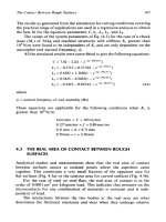
program is shown in Fig. 3.6 and good agreement can be seen. The rigid
body movement (0.66196
x
10-4 in.) was also found to compare favorably
with Mindlin's prediction (0.67 139
x
10-4
in.) with
a
deviation of 1.41
O/O.
EXAMPLE
2:
Circular Hertzian Contact with Different Materials.

The
contact
of
steel sphere of
I
in. radius on a rubber half space is considered.
The material constants used are as follows:
Tract ion
Disi
r
ibu
t
ion and Microslip in Frictional Contacts
x
103
35
30
25
5
0
0.0
0.2
0.4 0.6 0.8
1
.o
Scaled
Radius
(r/a)
69
Figure

3.6
the same material as compared with Mindlin's theory.
Traction distribution on the circular contact between two bodies
of
A
normal load of 2701bf, a tangential load of 361bf, and a coefficient of
friction of 0.2 are used in this case.
As
shown in Fig. 3.7, the traction distribution (symbol
s)
shows good
agreement with Mindlin's theory (solid line). The rigid body movement of
the rubber half space (0.39469
x
10-3in.) was found to be 30 times that of
the steel sphere (0.13156
x
10-4in.) and both agree well with Mindlin's
prediction with
a
2.29% deviation when a grid with
80
elements was used.
EXAMPLE
3:
Elliptical Hertzian Contact.
Four cases were investigated
in this example with different ratios between the major and minor axes
70
Chapter

3
Figure
3.7
Traction distribution on the circular contact between two bodies
of
differrent materials as compared with Mindlin’s theory.
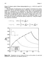
using different rectangular grid elements, as shown in Table 3.1.
A
Hert-
zian-type pressure distribution was assumed in all cases.
The results, which are plotted in Figs 3.8 to 3.1
1,
respectively, show
good agreement with Cattaneo’s theory
[
171. The rectangular grid elements
were used in order to save conveniently in computer storage. If a square grid
element had been used, better correlation would have been obtained.
The tangential force is applied in the direction of the a-axis in all cases.
Table
3.1
The Four Elliptical Hertzian Contact Cases
Contact area Number
of
grids Resulting figure
alb
=
2.0
a/b
=

0.5
a/b
=
8.0
a/b
=
0.125
112 Fig.
3.8
I12
Fig.
3.9
116 Fig.
3.10
I16
Fig.
3.11
x
103
0.0
0.2
0.4
0.6
0.8
1
.o
[i-]
Normalized
Distance
Figure

3.8
Traction distribution on the elliptical contact as compared with
Cattaneo’s theory
(a/b
=
2).
x
103
0.0
0.2
0.4
0.6
0.8
1
.o
Normalized
Distance
[
,/m]
Figure
3.9
Traction distribution on
the
elliptical contact as compared with
Cattaneo’s theory
(a/b
=
0.5).
x
103

0.0
0.2 0.4 0.6
0.8
1
.o
[/Em]
Normalized Distance
Figure
3.10
Traction distribution on the elliptical contact as compared with
Cattaneo’s theory
(a/h
=
8).
x
10’
0.0
0.2
0.4
0.6
0.8
[{Em]
Normalized Distance
0
Figure
3.1
1
Cattaneo’s theory
(a/b
=

0.125).
Traction distribution
on
the elliptical contact as compared with
Traction Distribution and Microslip in Frictional Contacts
73
EXAMPLE
4:
Square Contact Area
on
Semi-Infinite Bodies with Uniform
Pressure Distribution.
A
hypothetical square contact area between two
steel bodies with uniform contact pressure of
10,000
psi and a coefficient
of friction,
f
=
0.12, is discretized with 100 square grid elements. The
equal traction contours are shown in Figs
(3.12)
and
(3.13)
for a tangen-
tial force,
T
=
8001bf and 10001bf, respectively. The development of the

slip region with increasing tangential load and the rigid body movement is
shown in Figs.
3.14
and
3.15,
respectively.
EXAMPLE
5:
Discrete Contact Area
on
Semi-Infinite Bodies.
Two dis-
connected square areas of the same size (0.6in.
x
0.6in) on semi-infinite
steel bodies are
in
contact with uniform pressures assumed
on
each con-
tact region. The centroids of the two squares are placed 1.Oin. apart.
i
Traction
Contour
i
Distribution
+
430
psi
525

800
675
750
825
975
1080
1125
1200
mo
Figure
3.12
contact area
with
T
=
8001bf.
Contour plot of traction distribution on a uniformly
pressed
square
Chapter
3
i
Trac
on
i
Contour
;
Distribution
+
s30p.i

;
687
isss
i
972
i
143
i88
:
744
:
801
:
91s
:
1029
Figure
3.13
Contour plot of traction distribution on a
uniformly
pressed square
contact area
with
T
=
10001bf.
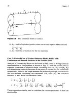
Three conditions of normal and tangential loading are used here:
Case 1.
PI
=

lO,OOOpsi,
P2
=
10,OOOpsi and the tangential load
is
Case 2.
Pi
=
20,OOOpsi,
P2
=
10,OOOpsi and the tangential load is
Case 3.
PI
=
20,OOOpsi,
P2
=
10,OOOpsi and the tangential load is
800
lbf applied at
45"
inclination.
800
lbf applied at
45"
inclination.
1200 lbf applied at
45"
inclination.

The coefficient of friction on both regions
1
and
2
is
assumed
to
be the same
wherefi
=f2
=
0.12.
The results for the three cases are given in Figs 3.16 to 3.18, respectively.
It can be seen in Case
1
(Fig.
3.16), that the traction contours and the slip
patterns are identical and the resultant traction force passes through the
centroid.
As
would be expected, the other two cases show different traction
distributions in the two disconnected contact areas and the resultant trac-
75
Figure
3.14
;ire3
with
incrensinf
tangential
load.

Development
of
slip
regions
on
a
uniformly
pressed
square contact
tian
force
is
consequently
found
to
be displaced from the centroid. The
effect
of
the tangential
load
on the
change
in
distribution
of
load
between
the
two
areas.

for the
case
with
region
1
and
2
subjected to norrnai pressures
of
2O.OOOpsi
and 1O.OOOpsi
respectively.
is
shown
in
Fig.
3.19a, and
the
location of
the
resultant force
for
each
area.
as
well
as
for
the
entire contact

area from the whole area centroid. is given
in
Fig.
3.19b.
An
illustration
of
76
1.2
1
.o
Chapter
3
8
0.6
L
b
0.0
0
1
2
3
4
5
Rigid
Body
Movement
(x
10-5
in.)

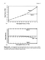
Figure
3.15
Tangential load versus rigid
body
movement curve for a uniformly
pressed square contact area.
the sequence
of
slip for the above case
is
shown in Fig.
3.20.
It can be seen
that, in this case, region
2
reached the condition
of
full slip at a load
of
1000 Ibf, whereas gross slip occurred for the total contact at 1296 lbf. Some
slip is also shown to occur in region
1
below l000lbf.
A
plot
of
the rigid
body movement versus the applied tangential load can be seen
in
Fig.

3.21
for the three considered cases.
3.4
FRICTIONAL CONTACTS SUBJECTED TO A TWISTING
MOMENT
3.4.1
Preprocessor
One of the boundary conditions,
in
this case, is that the direction
of
the
displacement in the no-slip region should be circumferential with respect to
the center of rotation on the contact surface
[23].
A preprocessor determines
the direction
of
the traction at each grid point by satisfying the above
Traction Distribution and Microslip in Frictional Contacts
77
r
I
I
I
I
I
I
I
I

I
I
I
I
I
I
I
I
I,
Figure
3.1
6
Traction distribution for contact
on
two discrete square areas under
an
8001bf
tangential load applied at a
45"
inclination.
PI
=
lO,OOOpsi,
P2
=
10,OOOpsi (Case
1).
boundary condition under the assumption of no slip
on
the entire contact

area to linearize the problem
[24].
This assumption implicitly implies that
the directions of discretized traction forces
will
not deviate significantly with
slip from those with no slip.
3.4.2
Problem
Formulation
For compatibility
of
deformation, the circumferential deformation should
be equal to the product of the angle of rigid rotation and the radial distance
78
Chapter
3
Tr
N
rotion
Contour
Di8tribution
700
Wt+
800
900
loo0
1100
1200
Tr

-action
Contour
Diutribution
700
Wit+
900
1100
1300
1500
1700
1900
2100
2300
f2
=
0.12
p2
=
20000 pui
Figure
3.1
7
Traction distribution for contact on two discrete square areas under
an 8001bf tangential load applied at
a
45"
inclination.
PI
=
20,00Opsi,

P2
=
10,000
psi
(Case
2).
from the center of rotation in the no-slip region and less than that in the slip
region. Because the bodies in contact are assumed to
obey
the law of linear
elasticity, the deformation at a grid point can be expressed as a linear super-
position of the effect of all the discretized traction forces acting on a contact
surface.
The traction force value should be less than the frictional resistance (the
product of the coefficient
of
friction and the normal force) in the no-slip
region and equal
to
the frictional resistance in the slip region.
For the equilibrium condition, the
sum
of the moment produced
by
the
discretized traction forces should be equal to the applied twisting moment.
Traction Distribution and Microslip in Frictional Contacts
79
Figure
3.1

8
Traction distribution for contact
on
two discrete square areas under
1200
Ib
tangential load applied at
a
45"
inclination.
P1
=
20,000
psi,
P2
=
10,000
psi
(Case
3).
Because the slip region is not known before hand, the complementary
condition (a
grid
point must be either in the no-slip region or in the slip
region) should be observed.
The problem is to find a set
of
the discretized traction forces which
satisfies all the above conditions with the assumed center
of

rotation. The
modified linear programming technique offers a readily suitable formulation
and
is
used to obtain the solution.