Friction and Lubrication in Mechanical Design Episode 1 Part 5 pptx

80
0.6
:
Region
2
0.5
0.4
Chapter
3
0.9
-
I
0.7:
o.o, , , , , , , , , ,.,,,., ,
0.0
0.1
0.2
0.3
0.4
0.5
0.6
0.7
0.8
0.9
1.0
1.1
1.2
1.3
(4
Total Applied
Force

(x
103
Ibf)
=
0.32
z
0.2:
6
-0.3:
-0.5
i
-0.4
1
=
0.3
0.1
z
0.2
6
-0.3:
-0.5
i
-0.4
1
Region
1
A-A-A-~A-A-A-~~A-A-A-A-A-A-~
(b)
Total Applied
Force

(x
10
Ibf)
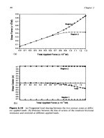
Figure
3.19
(a) Tangential load sharing between the two contact zones at differ-
ent applied loads. (b) Distance between the line
of
action
of
the resultant frictional
resistance and centroid at different applied loads.
Traction Distribution and Microslip in Frictional Contacts
81
f2=
0.12
p2=
10000
psi
/
f2=
0.12
p2=
20000
psi
500
600
700
800
900

650
1000
1Ox)
1100
1150
1200
1250 1280 1296
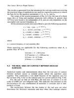
Figure
3.20
Development
of
slip regions on a discrete contact area with increas-
ing tangential load.
3.4.3
Iterative Procedure
The modified linear programming formulation is first implemented with an
initial guess for the center of rotation in order to find the discretized traction
forces whose directions are predetermined by the preprocessor. Now the
residual forces (the rectangular components of the sum of the traction
forces) can be calculated. These residual forces must be equal to zero
when the real center of rotation is found, since no tangential forces are
applied. The residual forces are then used to modify the center of rotation
and the process is repeated until the residual forces vanish. The real center of
rotation, the traction force distribution, the microslip region, and the angle
of
rigid body rotation are determined by this iterative procedure, as depicted
in the flow chart (Fig.
3.22).
82
Chapter

3
0.9
l.O,
0.8
1
1
LL-
5
0.4-
‘J.
5
0.3-
0.2-
F*
,., , ,
’.“(.’

.,
0.0 0.5
1
.o
1.5 2.0 2.5
3.0
RigM
Body
Movement
(xlW
in.)
(a)
1.4

1.2-
E.
&
1.0-
‘3
t
0.0
0.5
1.0
1.5
2.0
2.5
3.0
3.5
4.0 4.5
5.0
5.5
6.0
Rigid
Body
hV8ltWnt
(Xfw
in.)
(b)
Figure
9.21
(a) Joint compliance under same tangential loads before
gross
slip
(Case

1).
(b)
Joint compliance under different tangential loads before gross slip
(Cases
2
and
3).
Traction Distribution and Microslip in Frictional Contacts
b
83
forces
negligible?
Print
the results
Find the traction distribution
using the modified linear programming
Calculate the residual
force
c
Assume the new center
of
rotation
1
using a linear interpolation scheme
Figure
3.22
problem
subjected
to
a

twisting moment.
Flow
chart for the iterative procedure to solve frictional contact
3.4.4
Illustrative
Examples
EXAMPLE
1:
Circular Hertzian
Contact.
The contact between two steel
spheres of
1
in. radius (Fig. 3.23)
is
first considered in order to compare the
result from the developed procedure with the analytical solution by Lukin
[23]. The normal load is taken as 21601bf, the twisting moment is 2.45in.
-lbf, and the coefficient of friction is 0.1.
A
grid with 80 square elements is
used to discretize the circular contact area
of
0.36628
x
10-' in. radius.
A
comparison between Lubkin's theory (solid line) and the numerical
results (symbol
s)

is plotted in
Fig.
3.24 and very good agreement can be
seen. The angle of rigid rotation (0.10641
x
10-* rad) is also found to com-
pare favorably with Lubkin's theory (0.1
11
19
x
10-* rad) with a deviation
of 4.30%. The center of rotation is at the centroid.
84
Chapter
3
P
Ip
Figure
3.23
Contact
of
spherical bodies subjected to a twisting moment.
x
10’
Figure
3.24
Lubkin’s theory.
Traction distribution on the circular contact
as
compared

with
Traction Distribution and Microslip in Frictional Contacts
85
EXAMPLE
2:
Elliptical Hertzian Contact.
The elliptical Hertzian con-
tact area with an aspect ratio of
2
is assumed to occur when a normal
load of 21601bf is applied on two steel bodies. The pressure distribution is
assumed to be Hertzian in this case. The coefficient
of
friction is taken
to be equal to 0.1 and a twisting moment of 3.8in lbf is applied on the
interface.
A
grid with
80
rectangular elements of the side ratio of
2
is used
to discretize the elliptical contact area.
The contours of the magnitude and the direction of the tractions are
plotted in Figs. 3.25 and 3.26. The border line between the no-slip region
and the slip region
is
also shown
as
a

broken line. The centroid in this case is
the center of rotation.
Interpreted Magnitude
of
Stress
Figure
3.25
Contour plot
for
the magnitude
of
traction
on
the elliptical contact
area.
86
Chapter
3
Direction
of
Predirected Stress
(N=80)
Figure
5.26
Contour plot for the direction
of
traction on the elliptical contact.
EXAMPLE
3:
Disconnected Contact Areas

on
Semi-Infinite
Bodies.
Two
disconnected square areas of the same size (0.6in.
x
0.6in.) on a semi-
infinite steel body are assumed to be in contact with another semi-infinite
steel body. The centroids of the two squares are located
1
in. apart (Fig.
3.27). Uniform pressure is assumed on each contact region and the coeffi-
cient of friction is 0.12 for both regions. Two cases of normal loading are
considered here.
Case
1.
PI
=
10,OOOpsi and
P2
=
10,OOOpsi;
Case
2.
PI
=
20,OOOpsi
and
P2
=

10,OOOpsi.
Each region is discretized with 36 square elements to have 72 elements for
the entire contact area.
The contours of the magnitude and the direction of the tractions are
plotted in Figs 3.27 and 3.28 for Case
1
with a twisting moment of
500
in lbf
and in Figs 3.29 and 3.30 for Case 2 with a twisting moment of
700
in lbf. It
500
in-Ibfe
f,
=
0.12
P,
=
1000
psi
7
I
I
I
I
I
I
Figure
3.27

Contour plot for the
magnitude of traction on the contact
I
area of disconnected squares with
I
A4
=
500in lbf and normal loading of
Case
1.
I
I
f,
=
0.12 P,
=
10000 p8i
Figure
3.28
Contour plot
of
the
direction of traction on the contact area
of
disconnected squares with
M
=
500in lbf and normal loading
of
Case

I.
-1
70
600
inJM
@
f,
=
0.12
P,
=
IOOOO
psi
87
i
I
All
Slip
I
I
I
I
I
I
700 in-lbfQ f,
=
0.12 P, 20000
psi
-1
I

I
I
I
I
I
I
Figure
3.29
Contour plot for the
magnitude of traction on the contact
I
area of disconnected squares with
I
M
=
700in lbf and normal loading of
Case
2.
I
f,
=
0.12 Pz
=
10000
psi
+
700
in-Ibfo
f,
t

0.12 P,
=
20000 pai
Figure
3.30
Contour plot for the
direction of traction on the contact area
of disconnected squares with
M
=
700in lbf and normal loading of
Case
2.
88
Traction Distribution and Microslip
in
Frictional Contacts
89
can be seen that the traction contours and the slip patterns for both regions
1
and 2 are identical and the center
of
rotation is the centroid for the
symmetric normal loading.
As
would be expected, the case of asymmetric
normal loading shows different traction distributions in the two discon-
nected contact areas and the center of rotation is consequently found to
be displaced from the centroid. Also notice that region 2 reaches the state
of

total slip for Case 2, with a twisting moment of 700in lbf, and circumfer-
ential tractions are assumed for region
2.
The center
of
rotation always occurred on the line connecting the
centroids
of
two disconnected squares. The x-distance between the center
of rotation and the centroid for Case 2 versus the applied twisting moment is
plotted in Fig. 3.31.
The development of the slip region with the increasing twisting moment
is shown in Fig. 3.32 for Case 2. It can be seen that region
2
reaches a state
of
total slip at a twisting moment of 700 in lbf, and that gross slip occurs at
770 in lbf. Some slip is also shown to occur in region
1
below 700 in lbf.
The compliance curve relating the angle of rigid rotation and the twist-
ing moment is plotted in Fig. 3.33a
for
Case
1
and in Fig. 3.33b for Case 2.
0.40
0.0
0.1
0.2

0.3
0.4
015
0:s
017
0.8
1)
Twisting Moment
(xl
Oin-lbf)
Figure
3.31
twisting moments
on
the contact area of disconnected squares for Case
2.
Locations of the center of rotation from the centroid versus applied
90
Chapter
3
f,=
0.12
p2=
10000 psi
f,
=
0.12
p,
=
20000

psi
300
400
500 600
700
750
770
Figure
3.32
connected squares.
Progression of slip with increasing twisting for contact area of dis-
3.5
FRICTIONAL CONTACTS SUBJECTED TO A COMBINATION
OF TANGENTIAL FORCE AND TWISTING MOMENT
3.5.1
Iterative Procedure
The analysis
of
the frictional contact problem under a combination of tan-
gential force and twisting moment is a highly nonlinear problem. The
problem
is
piecewisely linearized using an iterative method and a modified
linear programming technique is utilized at each iteration. The procedure
followed in the iterative method is shown in Fig.
3.34.
Traction Distribution and Microslip in Frictional Contacts
91
0.7
b I I 1 l 1 1 1 1’7

0.0
0.5
1.0
1.5
2.0
2.5 3.0 3.5
4.0
(a)
Angk
d
Twist
(x10’
rat.)
0.8
-
m
l l , c
0
2 4
6
8 10
12 14
I
(b)
An@k
d
TM8t
@10*
nd.)
Figure

3.83
Compliance curve
for
the contact area
of
disconnected
squares:
(a)
Case
1;
(b)
Case
2.
3.5.2
Illustrative
Examples
EXAMPLE
1:
Circular
Hertzian
Contact.
The first example
is
an analy-
sis
of the contact between two
steel
spheres of 2in. radius (Fig.
3.35).
The

circular contact area of 5.15
x
10-2in. radius results from a normal load
of
30001bf
and the coefficient of friction
is
taken as
0.1.
The tangential
force
of
1461bf and the twisting moment of 4.8in lbf are applied
on
the
contact surface.
A
grid with
80
square elements is used to discretize the
circular contact area.
92
NO
<
Are
both
R:
and
RL
nealbiw?

>
Chapter
3
T'=R:
M1
=
R:,
Start
For
i
*
1,
initialize the discretized
traction at each grid
point
as zero
4
[
i=l+l
1
Find the
traction
distribution
due
to
the tangential
force
T'
using the
modified linear programming

[3]
fll
is the applied tangential
force)
Find the traction distribution due to
the twisting moment
M'
using the
preprocessor
and the modified linear
programming.
(M'
is the applied lwisting moment)
Combine the traction distribution due to
T'
and
Mi
with that
of
the previous iteration
1
1
1
Loop
100
for
ail the grid points
IS
the
combined traction

force
F:
bigger
than the limit value fP@t
a
grid point
k?
No
[Adjust
F:
to the limit
valuer^,
I
Calculate the residual
force
R:
and
the residual moment
RL
due to the
exceeding traction
forces
(F:
-
cp~)
Calculate the residual
force
R:
the residual moment
RL

due to
exceeding traction
forces
(F:
-
Figure
3.34
Flow
chart
for
the iterative procedure.
"P
-T
I
I'
T-
6"
1
Figure
3.35
force and twisting moment.
Contact of spherical bodies subjected to a combination of tangential
3.5
3.0
2.5
2
.o
1
.5
1

.o
0.5
3.5
3
.O
.)
2.5
2
.o
1
.s
1
.o
0.5
Figure
3.36
subjected to a combined load (using iterative procedure).
Contour plot
for
the magnitude
of
traction on the circular contact
93
94
Chapter
3
The contours
of
the magnitude and the direction
of

the traction distribution
using the iterative procedure are plotted in Figs 3.36 and 3.37. The border-
line between the no-slip region and the slip region is also shown as a broken
line. The center
of
rotation is found to be located at the centroid.
The rigid body movement and the angle of rigid rotation obtained by
the iterative procedure (0.68224
x
10-4
in. and 0.10670
x
10d2 rad) agree
well with those obtained by using a nonlinear programming formulation
[241*
The elapse
CPU
time on a Harris
800
to obtain the above results using
the iterative procedure is 14 min, whereas that using the nonlinear program-
ming technique is
31
min when the solution obtained by the iterative
procedure is used as an initial guess.
EXAMPLE
2:
Disconnected Contact Area
on
Semi-Infinite Bodies.

Consi-
der two disconnected square areas of the same size (0.6in.
x
0.6in.)
on
a
Figure
3.37
subjected
to
a combined load (using iterative procedure).
Contour plot for the direction of traction on the circular contact
Traction Distribution and Microslip in Frictional Contacts
95
semi-infinite steel body. The centroids of the two squares are located
1
in.
apart (Fig. 3.38). Uniform pressure is assumed on each contact region
and the coefficient of friction is 0.12 for both regions. Each region is dis-
cretized with 36 square elements (72 elements for the entire contact area).
Two cases of loading are considered here:
Case
1.
PI
=
20,000 psi,
P2
=
10,
!OOO

psi,
T
=
500
Ibf,
M
=
300
in lbf.
Case 2.
PI
=
lO,OOOpsi,
P2
=
20,OOOpsi,
T
=
6001bf,
M
=
400in lbf.
For Case
1,
the contours
of
the magnitude and the direction of the traction
distribution obtained by the iterative procedure are plotted in
Figs
3.38

and
3.39 and found to compare favorably with those obtained by applying the
nonlinear programming technique [24].
The corresponding results
for
Case 2 are shown in Figs 3.40 and 3.41. In
this case, region
1
is found to be in a state of total slip.
The
rigid body motions from the iterative procedure (0.16436
x
10F4 in.
and 0.12323
x
10-4rad for Case 1 and
0.30509
x
10-4in. and 0.32721
x
10-4rad for Case 2) compare favorably with those from the nonlinear
f,
=
0.12
e,
=
loo00
f,
-
0.12

P,
=
20000
pi
Figure
3.38
Contour plot for the magnitude of traction on the contact area of
disconnected squares for Case
1
(using iterative procedure).
f2=0.12 P*rlOO00pd
midM
+M)OIbf
f,
=
0.12
P,
=
20000
pcri
Figure
3.39
Contour plot for the
direction of traction on the contact
area of disconnected squares for Case
1
(using iterative procedure).
f2
=
0.12

P,
=
20000
psi
400
in4M
+6OOIM
*
I
I
Uniform-
I
Figure
3.40
Contour plot for the
:
str~s-12~psi
:
magnitude
of
traction on the contact
area
of
disconnected squares for Case
2
(using iterative procedure).
I
I
I
I

:
I
:

J
96
Traction Distribution and Microslip in Frictional Contacts
97
f,
=
0.12
P,
=
20000
psi
4oo
in,M
-6OOIW
f,
=
0.12
P,
=
10000
psi
Figure
3.41
disconnected squares for Case
2
(using iterative procedure).

Contour plot for the direction
of
traction on the contact area of
programming technique (0.16502
x
10-4 in. and
0.12263
x
10-4
rad for
Case
1
and
0.31257
x
10-4in. and
0.30892
x
10-4rad for Case
2),
with
deviations of
2.39%
and
0.49%
for Case 1, and
2.31%
and
5.92%
for

Case
2,
respectively.
The elapse CPU times on a Harris
800
to obtain the above results by the
iterative procedure are
2
min for Case
1,
and
8
min for Case
2,
whereas those
necessary to obtain the results from the nonlinear programming technique
are 18 min for Case
1,
and 46
min
for Case
2,
respectively, when the solu-
tions obtained by the iterative procedure are used as initial guesses.
REFERENCES
1.
Hertz, H., “Miscellaneous Papers” translated
by
Jones,
D.

E.,
and Schott,
G.
A.,
Macmillan, New York, NY,
1896,
pp.
146162,
163-183.
2.
Lundberg,
G.,
“Elastische Beruhrung Zweier Halbraume,”Forsch.
Ingenieurw., 1939, Vol.
10,
pp.
201-21
1.
98
Chapter
3
7.
8.
9.
10.
11.
12.
13.
14.
15.

16.
17.
18.
19.
Cattaneo, C., “Teoria del contatto elasiico in seconda approssimazione,”
University of Rome, Rend., Mat. Appl., 1947, Vol. 6, pp. 504-512.
Conway, H. D., “The Pressure Distribution between
Two
Elastic Bodies in
Contact,”
2.
Angew. Math. Phys., 1956, Vol. 7, pp. 460-465.
Greenwood, J. A., and Tripp, J. H., “The Elastic Contact of Rough Spheres,”
J. Appl. Mech., Trans. ASME, March 1967, pp. 153-159.
Schwartz, J., and Harper, E.
Y.,
“On the Relative Approach of Two
Dimensional Elastic Bodies in Contact,” Int. J. Solids Struct., Dec. 1971,
Tsai, K. C., Dundurs,
J.,
and Keer, L. M., “Contact between an Elastic Layer
with a Slightly Curved Bottom and a Substrate,” J. Appl. Mech., Trans.
ASME, Sept. 1972, Ser. E., Vol. 39(3), pp. 821-823.
Kalker, J. J., and Van Randen,
Y.,
“Minimum Principle for Frictionless Elastic
Contact with Application to Non-Hertzian Contact Problems,”J. Eng. Math.,
April 1972, Vol. 6(2), pp. 193-206.
Conry, T.
F.,

and Seireg, A., “A Mathematical Programming Method for
Design of Elastic Bodies in Contact,” J. Appl. Mech., Trans. ASME, June
Erdogan,
F.,
and Ratwani, M., “Contact Problem for an Elastic Layer
Supported by Two Elastic Quarter Planes,” J. Appl. Mech., Trans. ASME,
Sept. 1974, Ser. E, Vol. 41(3), pp. 673-678.
Nuri,
K.
A.,
“Normal Approach between Curved Surfaces in Contact,” Wear,
Francavilla, A., and Zienkiewicz,
0.
C., “Note
on
Numerical Computation of
Elastic Contact Problems,” Int. J. Numer. Meth. Eng., 1975, Vol. 9(4), pp.
Haug, E., Chand,
R.,
and Pan,
K.,
“Multibody Elastic Contact Analysis by
Quadratic Programming,”
J.
Optim. Theory Appl., Feb. 1977, Vol. 21(2), pp.
Kravchuk, A.
S.,
“On the Hertz Problem for Linearly and Non-Linearly
Elastic Bodies of Finite Dimensions,” Appl. Math. Mech., 1977, Vol. 41(2),
pp. 320-328.

Goriacheva,
I.
G., “Plane and Axisymmetric Contact Problems for Rough
Elastic Bodies,” Appl. Math. Mech., 1979, Vol. 43(1), pp. 104-1 11.
Mindlin,
R.
D.,
“Compliance
of
Elastic Bodies in Contact,” J. Appl. Mech.,
Trans. ASME, 1949, Vol. 16, pp. 259-268.
Cattaneo, C.,
“Sul
Contatto di due Corpi Elastici: Distribuzione Locale Degli
Sforzi,” Accad. Lincei, Rendic., 1938, Ser.
6,
Vol. 27, pp. 342-348, 434-436,
474-478.
Johnson,
K.
L., “Surface Interaction Between Elastically Loaded Bodies
Under Tangential Forces,” Proc. Roy. Soc. (Lond.), 1955,
A,
Vol. 230, pp.
Deresiewicz, H., “Oblique Contact of Non-Spherical Elastic Bodies,” J. Appl.
Mech., Trans. ASME, 1967,
Vol.
24, pp. 623-624.
Vol. 7(12), pp. 1613-1626.
1971, pp. 387-392.

Dec. 1974, Vol. 30(3), pp. 321-335.
9
1
3-924.
189-198.
531-548.
Traction Distribution and Microslip in Frictional Contacfs
99
20.
21.
22.
23.
24.
Danzig, G.
W.,
Linear Programming and Extensions, Princeton University
Press, Princeton, NJ, 1963.
Love, A. E. H., A Treatise on the Mathematical Theory of Elasticity, 4th ed.,
Dover Book Company, New York, NY, 1944.
Timoshenko,
S.
P.,
and Goodies,
J.
N., Theory of Elasticity, 3rd ed., McGraw
Hill Book Company, New York, NY, 1970.
Lubkin, J. L., “The Torsion of Elastic Spheres in Contact,”
J.
Appl. Mech.,
Trans. ASME, 1951, Vol.

73,
pp. 183-187.
Choi, D., “An Algorithmic Solution for Traction Distribution in Frictional
Contacts,” Ph.D. Thesis, The University of Wisconsin-Madison, 1986.
The Contact
Between
Rough
Surfaces
4.1
SURFACE ROUGHNESS
All surfaces, natural or manufactured, are not perfectly smooth. The
smoothest surface in natural bodies is that of the mica cleavage. The mica
cleavage has a roughness of approximately 0.08pin. The roughness
of
manufactured surfaces vary from a few microinches to
1000
pin. depending
on the cutting process and surface treatment. Representative examples of
some of these are given in Table 4.1.
Roughness represents the deviation from a nominal surface and is
a
composite of waviness and asperities. Both of these are shallow curved
surfaces with the latter having wavelengths orders
of
magnitude smaller
than the former. Asperities can be also considered as wavy surfaces
on
a
microscale with their height being in the order of
2-5%

of the wavelength,
as illustrated in Fig. 4.1.
4.2
SURFACE ROUGHNESS GENERATION
Surface roughness plays an important role in machine design. During the
metal cutting operation, a machined surface is created as a result of the
movement of the tool edge relative to the workpiece. The quality of the
surface is a factor
of
great importance in the evaluation of machine tool
productivity. The results from a large number of theoretical and experi-
mental studies on surface roughness during turning are available in the
100
The
Contact Between
Rough
Surfaces
10
I
Table
4.1
Processes
Average Surface Roughness for Some Common Manufacturing
~~~~~~
Manufacturing process
Average surface roughness (pin.)
Super finishing
Lapping
Polishing
Honing

Grinding
Electrolytic grinding
Barrel finishing
Boring, turning
Die casting
Cold rolling, drawing
Extruding
Reaming
Milling
Mold casting
Drilling
Chemical milling
Elect. discharge machining
Planing, shaping
Sawing
Forging
Snagging
Hot rolling
Flame cutting
Sand casting
2-8
2-16
4-16
4-32
4-63
8-16
8-32
16-250
32-63
32-125

32-1
25
32-125
32-250
63-1 25
63-250
63-250
63-250
63-500
63-1000
125-500
250-1
000
500-
1000
500-
1000
500-
1000
literature
[
1-18].
Although various factors affect the surface condition
of
a
machined part, it is generally accepted that the cutting parameters such as
speed, feed, rate, depth
of
cut, and tool nose radius have significant influence
on the surface geometry for

a
given machine tool and workpiece setup.
There is also general agreement that surface roughness improves with
increasing machine tool stiffness, cutting speed, and
tool
nose
radius, and
decreasing feed rate
[l-31.
It has also been reported
[2,
91
that at speeds less
than a certain value, discontinuous
or
semidiscontinuous chips and built-up-
edge formation may occur, which can give rise to poor surface finish. At
speeds above that specific value, the built-up-edge size decreases and the
surface finish improves. This specific speed limit depends on many factors
such as workpiece, tool conditions, and the state of the machine tool. Sata
[9]
reported
22.86
m/min as the speed limit in his experiment. Of the factors
influencing the surface roughness, the depth of cut was found to have the
102
Chapter
4
Figure
4.1

modification.
(a) Profile
of
surface roughness.
(b)
Asperity curvature without height
least effect. Statistical techniques, developed by Box and Wilson, have been
applied to establish a predictive equation for the relationship between
tool
life or surface roughness and cutting conditions
[6,
7,
191.
Other studies indicated that tool wear causes the surface finish to dete-
riorate rapidly and has a direct effect on the maximum roughness
[4].
Also,
the principal cutting edge and hardness of the workpiece material itself are
found to affect the surface roughness
[5,
201.
Some studies presented sto-
chastic models to characterize the indeterministic components of surface
texture
[
16,
201.
For
a
tool with

a
finite radius in an idealized cutting condition with
a
rigid machine tool, the peak-to-valley roughness,
Rmax,
which is known as
kinematic roughness, in the case of small values of feed can be shown to
be
[
141:
f2
R,,,
=
for
f
5
2r
sin
Do
(4.1)
The Contact Between Rough
Surfaces
103
where
R,,,
=
peak-to-valley surface roughness
f
=
feed rate

r
=
tool radius
De
=
end relief angle
Based on an extensive experimental study using one lathe, Hasegawa et al.
[8]
developed a statistical relationship of peak-to-valley surface roughness,
R,,,
in terms of the cutting speed, feed rate, depth of cut, and tool nose
radius using a response surface method. The statistical relationship is given
approximately by the following:
(4.2)
where
v
=
cutting speed
d
=
depth
of
cut
It can be seen that considerable variations in the calculated surface rough-
ness may result from the use
of
Eqs
(4.1)
and
(4.2),

as well as any of the
numerous empirical equations available in the literature
[l-81.
One
of
the
main reasons for the discrepancies is that the vibratory behavior is defined
by the relative movement of the tool with respect to the workpiece in the
machining process and has deterministic and stochastic components.
As
reviewed above, the stochastic component is assumed
to
be the results of
the random excitation during the cutting process and the deterministic com-
ponent depends on the dynamic characteristics of the machine tool. In order
to select or modify a machine tool, which can be used to generate a parti-
cular surface quality, it is necessary to quanfity the influence of its dynamic
parameters on surface roughness [21-281.
A
piecewise dynamic simulation of the interaction between the tool and
the workpiece system in turning is reported by Jang and Seireg
[29].
A
generalized computer-based model is developed for predicting surface
roughness for any given condition which takes into consideration all the
important parameters influencing the deterministic vibratory behavior
of
the
machine tool-workpiece system. The parameters considered in the simula-
tion are: the feed rate, cutting speed, depth of cut, radius of cutting edge, the

dimensions of the workpiece, and the mass, stiffness, and damping of the
machine structure as well as the cutting tool assembly.
104
Chapter
4
Extensive numerical results from the simulation suggest that the
uncoupled natural frequency of the tool assembly is the fundamental para-
meter controlling the generated surface roughness. The parametric equation,
which is developed from the simulation results, is found to be in good
agreement with the data obtained from an extensive series of tests using
mild steel specimens. The simulation results also show that the well-
known kinematic equation for predicting surface roughness based on the
geometry of the cutting process gives essentially the same results as the
simulation when the tool natural frequency is greater than
150
Hz.
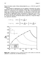
Figure
4.2
gives a sample result from the simulation.
It
shows the aver-
age generated surface roughness along the generatrix of the workpiece. The
roughness values were obtained
by
displacing the tool edge an amount equal
to the sum
of
the average relative vibration at each axial location and the
kinematic roughness.
The simulation was utilized

to
develop generalized equations for surface
roughness based on the output from the vibratory model.
A
generalized
equation
of
the following form
is
assumed:
Distance
Along
Workpiece
(mm)
2
Figure
4.2
Average surface roughness along the axis
of
workpiece
(V
=
61
m/
min,
f'
=
0.127 mmlrev,
d
=

0.305 mm,
r
=
0.794 mm).
(.)
W
=
34 Hz,
(0)
W
=
28
Hz.