Friction and Lubrication in Mechanical Design Episode 1 Part 8 pdf

Thermal Considerations in Tribology
155
O.Oo80
I
I
I
I
I
I
I
I
I
Lubricated
-
d0Wr solid

Dry
-
both
80lid
8UrfaGW

0.0075
-
-
Lubrlcated
-
faster 80lld
A
0
/

0
0
4
q
=
~-in/in*-s
=
frictional
power
intensity
0
0
0
0
0
-
0.0070
-
T-r'F
0
0
-
0
0
1
0
0
5
0
0

&
0.0065
-
c
0
0
#
0
-
0
#
0
0
0
*
40-
0-
p'
i
O.Oo60
-
0 0-
I-
=.
7-7

*
\
____
.__

-
*
-
0.0055
-
-
0.0050
I
I
I
I
I
I
I
I
I
1
I
I
I
I
.
0.0
0.2
0.4
0.6
0.8
1
.o
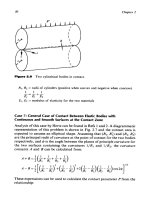
siderable difference between the film and solid temperatures. Figure

5.27
represents the case of a metallic solid with an insulative surface layer in
contact with another layered solid having an opposite combination of ther-
mal properties. It can be seen from the figure that the heat partition is highly
dependent on the ratio
Hd/H,,
where
h02
+
ho1
Hd
=
h2 -hol
and
H,,
=-
2
The latter is kept constant to show the main influence of the difference in
surface layer thicknesses. The existence of surface layers strongly deviated
the heat partition from the dry sliding condition. This phenomenon could be
explained by the cooling mechanism in the contact zone by a shallow region
near the surface, which mainly incorporates the layer thickness. Figure
5.27
also demonstrates the possibilities for equalizing the heat partition between
the moving solids by controlling both thermal properties and thicknesses
of
surface layers. Negligible sliding is assumed in this case.
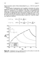
Figure
5.28
shows the variation in the maximum temperature rise in the

contact zone and the solid surfaces with respect to
Hd/Haw.
The contact
I
I
I
I
I
I
I
I
I
1
1
Film
Slower
Surface
Fader
Surface


8 10
12
14 16 18
20
P,
(1
0'
psi)
Figure

5.26
Maximum temperature rise versus maximum pressure for
50%
slid-
ing (steel-oil-steel, rolling velocity
=
400
in./sec,
RI
=
R2
=
1
in.).
0.4
0.3
-1
.o
-0.5
0.0
0.5
1
.o
Ha
'
H,
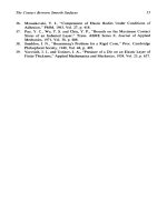
Figure
5.27
Heat partition versus
Hd/H,,,,

(rolling velocity
=
2000
in./sec,
1=.02
in.,
K~=K~~,
K~~=K*=.I
K~,
H,,,=~o~
in.).
Thermal Considerations in Tribology
IS
7
0.0080
A
0.0057
z
E
E
d
>
0.0033
-
0.M)lO
-1
.o
-0.5
0.0
0.5

1
.o
H*'H,
Figure
5.28
KI
=
KO2,
Kol
=
K2
=
.I
K1, Ha,,
=
104 in.).
Tmax/q,
versus
Hd/Hm(rolling speed
=
2000
in./sec,
1
=
.02
in.,
zone temperature is almost identical to the solid surface temperature, which
carries the conductive surface layer.
The generalized equation for heat partition in lubricated line contact
problems, which has been derived for steady-state conditions, is applicable

to all metallic solids. It can be deduced from this equation that the deviation
in heat partition from that calculated
by
Jaeger and Blok is highly influenced
by the conductivity and thickness of the lubricant film. The existence of the
lubricant film tends to equalize heat partition between the rolling/sliding
solids independent of their thermal properties and surface speeds. It is inter-
esting to note that the maximum temperature rise for each moving solid is
directly proportional to the heat partition coefficient,
yl,
y2,
the ratio of the
trailing edge penetration depth to thermal conductivity,
D1
/kl,
D2/k2,
and
the total heat flux,
q,/l.
The difference between the maximum film and surface temperatures is
also controlled by the lubricant film thickness and its conductivity. This can
be attributed to the fact that convection
is
not important in this case.
Although the problem of layered surfaces is appropriately modeled in
the developed finite difference program, an evaluation of the effect of the
different system parameters on the temperature distribution would be extre-
mely difficult. It was, therefore, imperative to limit the parametric analysis
I58
Chapter

5
to single layered solids for two specific regimens of thermal properties, layer
thicknesses, width of contact and operating speeds.
The following can be concluded from the dimensionless equations
developed for the considered cases:
1.
The surface temperature of the solid decreases with increasing con-
ductivity of the layers and their thickness due to the convection
influence under such conditions.
For conductive surface layers, the slide/roll ratio has little influence
on the maximum solid surface temperatures, while for insulative
surface layers, the slide/roll ratio has a significant influence on the
maximum temperature.
For conductive surface layers with equal thicknesses, increasing the
thickness decreases the maximum surface tempratures for both the
solid and the surface layers.
For insulative surface layers with equal thicknesses, increasing the
thickness slightly decreases the maximum solid surface tempera-
tures and increases the maximum surface layer temperatures.
For a conductive solid,
kl,
with an insulative surface layer,
kol,
contacting an insulative solid,
k2,
with conductive layer,
k02,
assuming that
kl
=

k02
and
k2
=
kol,
there is a signficant deviation
of the partition from the unlayered case, as shown in Fig.
5.27.
It
can also be seen that with the above combination of properties it is
possible to attain equal heat partition by proper selection of the
layer thicknesses (at
Hd/Have
=
-0.325
in this case).
For the above case, the maximum contact temperature is approximately
equal to the maximum temperature in the insulative solid with conductive
layer for all thickness ratios (Fig.
5.28).
The maximum temperature for the
conductive solid with insulative layer is significantly lower than the interface
temperature.
2.
3.
4.
5.
REFERENCES
1.
Cheng,

H.
S.,
“Fundamentals
of
Elastohydrodynamic Contact Phenomena,”
International Conference on the Fundamentals
of
Tribology, Suh,
N.
and
Saka,
N.,
Eds., MIT Press, Cambridge, MA, 1978,
p.
1009.
Blok,
H.,
“The Postulate About the Constancy of Scoring Temperature,”
Interdisciplinary Approach
to
the Lubrication
of
Concentrated Contacts,
P.
3.
Sakurai, T., “Role
of
Chemistry in the Lubrication of Concentrated
2.
M.

Ku,
Ed., NASA SP-237, 1970, p.
153.
Contacts,” ASME
J.
Lubr. Technol.,
1981,
Vol. 103, p. 473.
Thermal Considerations in Tribology
159
4.
5.
6.
7.
8.
9.
10.
11.
12.
13.
14.
15.
16.
17.
18.
19.
Alsaad, M., Blair,
S.,
Sanborn,
D.

M., and Winer, W.
O.,
“Glass Transitions
in Lubricants: Its Relation to EHD Lubrication,” ASME J. Lubr. Technol.,
1978, Vol. 100,
p.
404.
Blok, H., “Theoretical Study
of
Temperature Rise at Surfaces of Actual
Contact Under Oiliness Lubricating Conditions,” Proc. Gen. Disc.
Lubrication, Institute of Mechanical Engineers, Pt. 2, 1937, p. 222.
Jaeger,
J.
c., “Moving Sources
of
Heat and the Temperature at Sliding con-
tacts,” Proc. Roy. Soc., N.S.W., 1942, Vol.
56,
p. 203.
Cheng,
H.
S.,
and Sternlicht,
B.,
“A Numerical Solution for the Pressure,
Temperature, and Film Thickness Between Two Infinitely Long, Lubricated
Rolling and Sliding Cylinders under Heavy Loads,” ASME J. Basic Eng., Vol.
87, Series
D,

1965, p. 695.
Dowson, D., and Whitaker, A.
V.,
“A Numerical Procedure for the Solution
of the Elastohydrodynamic Problem of Rolling and Sliding Contacts
Lubricated by a Newtonian Fluid,” Proc. Inst. Mech. Engrs, Vol. 180, Pt.
3, Ser. B, 1965, p. 57.
Manton, S. M., O’Donoghue,
J.
P.,
and Cameron, A., “Temperatures at
Lubricated Rolling/sliding Contacts,” Proc. Inst. Mech. Engrs, 1967-1 968,
Vol. 1982, Pt. 1, No. 41, p. 813.
Conry, T.
F.,
“Thermal Effects on Traction in EHD Lubrication,” ASME J.
Lubr. Technol., 1981, Vol. 103, p. 533.
Wang,
K.
L., and Cheng, H.
S.,
“A
Numerical Solution to the Dynamic Load,
Film Thickness, and Surface Temperatures in Spur Gears; Part
1
Analysis,”
ASME J. Mech. Des., 1981,
Vol.
103,
p.

177.
Knotek,
O.,
“Wear Prevention,” International Conf. on the Fundamentals of
Tribology, Suh, N., and Saka, N., Eds., MIT Press, Cambridge,
MA,
1978,
p.
927.
Torti, M. L., Hannoosh, J.
G.,
Harline,
S.
D., and Arvidson, D. B., “High
Performance Ceramics for Heat Engine Applications,” AMSE Preprint No.
Georges, J. M., Tonck, A., Meille,
G.,
and Belin, M., “Chemical Films and
Mixed Lubrication,” Trans. ASLE, 1983, Vol. 26(3), p. 293.
Poon,
S.
Y.,
“Role of Surface Degradation Film on the Tractive Behavior in
Elastohydrodynamic Lubrication Contact,” J. Mech. Eng. Sci., 1969, Vol.
I1(6), p. 605.
Berry, G. A., and Barber, J.
R.,
“The
Division of Frictional Heat
-

A guide to
the Nature of Sliding Contact,” ASME J. Tribol., 1984, Vol. 106, p. 405.
Shaw, M. C., “Wear Mechanisms in Metal Processing,” Int. Conf. on
the
Fundamentals
of
Tribology,
Suh,
N., and Saka, N., Eds., MIT Press,
Cambridge, MA., 1978,
p.
643.
Burton,
R.
A., “Thermomechanical Effects on Sliding Wear,” Int. Conf. on
the Fundamentals of Tribology, Suh, N., and Saka,
N.,
Eds., MIT Press,
Cambridge, MA., 1978, p. 619.
Ling,
F.
F.,
Surface Mechanics,
J. Wiley, New York,
NY,
1973.
84-GT-92, 1984.
160
Chapter
S

20.
21.
22.
23.
24.
25.
26.
27.
28.
29.
Klaus, E. E., “Thermal and Chemical Effects in Boundary Lubrication,”
Lubrication Challenges in Metalworking and Processing, Proc.
1
st Int.
Conf., IIT Res. Inst., June, 1978.
Winer, W.
O.,
“A Review of Temperature Measurements in EHD Contacts,”
5th Leeds-Lyon Symposium, 1978, p. 125.
Townsend,
D.
P.,
and Akin, L.
S.,
“Analytical and Experimental Spur Gear
Tooth Temperature as Affected by Operating Variables,” ASME J. Lubr.
Technol., 1981, Vol. 103, p. 219.
Rashid,
M.,
and Seireg, A., “Heat Partition and Transient Temperature

Distribution in Layered Concentrated Contacts. Part
I
:
Theoretical Model,
Part
2:
Dimensionless Relationships, ASME J. Tribol., July 1987, Vol. 109,
p.
496.
Taylor, E.
S.,
Dimensional Analysis for Engineers,
Oxford University Press,
London, England, 1974.
David,
F.
W., and
Nolle,
H.,
Experimental Modeling in Engineering,
Butterworths, London, England, 1974.
Arpaci, V.
S.,
Conduction Heat Transfir,
Addison-Wesley, Reading,
MA,
1966, p. 474.
Hamrock, B.
J.,
and Jacobson, B.

O.,
“Elastohydrodynamic Lubrication
of
Line Contacts,” ASLE Trans.,
1984,
Vol.
27,
p.
275.
Wilson,
W.
R. D., and Sheu,
S.,
“Effect on Inlet Shear Heating Due
to
Sliding
on Elastohydrodynamic Film Thickness,” ASME J. Lubr. Technol., 1983,
Vol. 105, p. 187.
Suzuki, A., and Seireg, A., “An Experimental Investigation of Cylindrical
Roller Bearings Having Annular Rollers,”
ASME
J. Lubr. Technol., 1976,
Vol. 98, p. 538.
6
Design
of
Fluid
Film
Bearings
6.1

HYDRODYNAMIC
JOURNAL
BEARINGS
Fluid film bearings are a common means of supporting rotating shafts in
rotating machinery. In such bearings
a
pressurized fluid film is formed with
adequate thickness to prevent rubbing of the mating surfaces. There are two
main types
of
fluid film bearings: hydrostatic and hydrodynamic. The first
type relies on an external source
of
energy to supply the lubricant with the
necessary pressure. In the second type, pressure is developed within the
bearing as a result
of
the relative motion between shaft and bearing. The
pressure is influenced by the geometry
of
the fluid wedge, which is formed to
sustain the load, as illustrated in
Fig
6.1.
6.1.1
Hydrodynamic Equations
The basic equation governing the behavior
of
the fluid film in the hydro-
dynamic case is Reynolds’ equation

[
I].
Assuming isothermal, incompressi-
ble flow this equation is derived by consideration of the Newtonian shear
-
velocity gradient relationship, the equilibrium
of
the fluid element (Fig.
6.2)
in the
x-
and z-directions and the continuity equation. Accordingly:
161
162
W
Chapter
6
Figure
6.1
Bearing geometry.
where
p
=
film pressure
h
=
film thickness
p
=
oil viscosity (assumed constant throughout the film)

U
=
tangential velocity in the journal
The solution
of
this equation for any eccentricity,
e,
would result in expres-
sions for the quantity
of
flow required, the frictional power loss and the
pressure distribution in the oil film. The latter determines the load-carrying
capacity of the bearing.
A
closed-form solution of Reynolds’ equation can
be obtained with either of the following assumptions:
1.
Assume the bearing to be long compared to its diameter. This is
generally known as the Sommerfeld bearing. In this case the
change in pressure in the axial direction can be neglected
com-
pared to the change in the circumferential
(x)
direction.
Accordingly:
Design of Fluid
Film
Bearings
Y
2

de
ay
ax
sdx dy dz =-dx dy dt
Figure
6.2
Equilibrium
of
fluid element in
the
x-direction.
and
Eq.
(6.1)
reduces
to:
Referring to Fig.
6.1
with the condition:
163
dy dr
p=pmax
at
h
=
hl
164
Chapter
6
and

p=po
at
8=0
and 8=2n
Equation
(6.2)
can be integrated
to
yield:
2C(1
-
E*)
2
+
E2
hi
=
6p
UR
!)=PO+-
E
sin
8(2
+
E
cos
0)
c*
((2
+

&2)(1
+
ECOSO)
12XE
F
(s)
-
4n(l
+
2~~)
-
PLU
R
2+&2Ji-z2
(6.3)
(6.4)
(6.5)
where
W
=
bearing load
F
=
tangential load
h,
=
film thickness at peak pressure
C
=
radial clearance

R
=
radius
of
the bearing
E
=
=
eccentricity ratio
8
=
angle measured from negative direction of x-axis (rads)
C
Equation
(6.5)
can be rewritten in terms
of
a dimensionless num-
ber,
S,
called the Sommerfeld number:
(2
+
S=
12dE
so
that
s
=
-(-)*=

pUL
R
R
'pN
p
nW
c
where
N,
P
=journal rotational speed and average pressure, respectively
Design
of
Fluid Film Bearings
165
2.
The bearing length
is
small compared to its diameter. The ana-
lysis of this case is called the
short bearing approximation.
The
flow in the axial
(2)
direction is assumed to
be
considerably
greater than that in the circumferential direction. Accordingly,
Reynolds' equation reduces
to

with
the
boundary conditions:
L
2
z=-
p=O
at
where
L
=
bearing length
The solution
of
Eq.
(6.9)
yields:
($2)
(1
+
E
COS
q3
&dx2(1
-
E*)
+
16c2
pULR
2n

F=(7)-
(6.9)
(6.10)
(6.11)
(6.12)
(6.13)
where
4
=
attitude angle between the load line and the line
of
enters
D
=journal diameter
Equation (6.1
1)
can be rewritten in terms
of
the Sommerfeld
number,
S,
as:
(1
-
E2y
2
'(i)
=
m,/z2(1
-

E~)
+
16~~
(6.14)
166
Chapter
6
6.1.2
Numerical Solution
The development of high-speed computers made it possible to obtain
numerical solutions for Reynolds’ equation
(6.
I).
Accordingly, bearing
behavior can be calculated for any given geometry and boundary condi-
tions. The numerical results of Raimondi and Boyd
[2-4]
are among the
most widely known. Their data are presented in the form
of
design charts
with Sommerfeld number as the main parameter. The numerical solutions
are based on the assumption of an isoviscous film independent
of
pressure
and temperature variations. The film viscosity is calculated at the mean
temperature in the bearing. The bearing performance charts
of
Raimondi
and Boyd are given in Figs

6.3-6.7.
6.1.3
Equations for Predicting Bearing Performance
A
system of equations, based on these charts, is developed by approximate
curve fitting. The equations are utilized in the automated design system
described later in this chapter. These equations are:
0.01
I
L
I
A
0.01
0.1
1
Sommerfeld
Number,
S
Figure
6.9
Minimum film thickness.
0-L
Volume
Flow
Variable,
Q/(
RNCL)

0
Friction Coefficient,

F=
f
x
(Wc)
b
I
1
.
.
1
I
168
Chapter
6
Sommerfeld
Number,
S
Figure
6.6
Peak pressure.
J
=
Joule'r equivalent
of
heat
t
1
0.01 0.1
1
I

I
Sommerfeld
Number,
S
Figure
6.7
Temperature variable.
Design
of
Fluid Film Bearings
1.2.
2.0.
2.1.
169
170
Chapter
6
The following notation is used in the analysis:
C
=
radial clearance (in.)
D
=journal diameter (in.)
e
=journal eccentricity (in.)
f
=
coefficient of friction
ho
=

minimum film thickness (in.)
L
=
bearing length (in.)
N
=journal rotational speed
(rps)
P
=
bearing average pressure (lb/in.2)
P,,,
=
maximum oil film pressure (lb/in.2)
Q
=
quantity of oil fed to bearing (i~~.~/sec)
R
=journal radius (in.)
At
=
oil temperature rise
(OF)
W
=
bearing load (Ib)
p
=
lubricant average viscosity (reyn)
4
=

attitude angle
I,,,
=
maximum
oil
film temperature
(OF)
Dimensionless groups:
R
RNCL
L
D
S=
f
c=

-
Q
-=
frictional variable
oil
flow
variable
length to diameter ratio
P
Sommerfeld no.
=
6.1.4
Whirl
and Stability Considerations

The whirl of rotors supported on fluid films is of considerable practical
importance and it is no surprise that
it
has been the subject of numerous
investigations. The designer
is
generally interested in predicting beforehand
not only the stability of the rotor operation but the expected peak amplitude
of
whirl orbit at a given operating speed resulting from a particular amount
of
unbalance. The safety during the transient start-up phase has to be also
Design
of
Fluid Film Bearings
I71
insured. Some
of
the excellent contributions to the analysis
of
this problem
and related bibliographies can be found in Refs 5-12.
A
simplified stability criterion, based on an analysis by Lund and Saibel
[Ill, is also given in Fig.
6.8.
A
modified Sommerfeld number,
CT
=

YTS(L/D)~,
and a dimensionless rotor mass,
MCw2/W,
determines the
condition for the onset of bearing instability according to the relationship
plotted in the figure, where
M
=
rotor mass per bearing
C
=
radial clearance
w
=journal rotational speed (rad/sec)
W
=
bearing load
Mathematical expressions describing the limits of journal stability as
a
func-
tion
p
of
CT
can be derived from Fig.
6.8
as:
CJ
5
0.28:

~(cT)
=
3/0'.~~
0.28
5
CJ
5
2.90:
p(a)
=
6.880.~''~~
CJ
>
2.90:
p(a)
=
7.65
1.
2.
3.
6.1.5
The Effect
of
Rotor Unbalance on Whirl Amplitude and Stability
It is well known that rotor unbalance can have significant effect on whirl
and stability.
A
study by Seireg and Dandage [13] utilized the phase-plane
method to simulate the dynamics
of

an unbalanced rotor supported by an
isoviscous film. Response spectra were obtained to illustrate the trend
of
the
influence of the magnitude of unbalance, speed, average film viscosity, load,
clearance, and rotor start-up, acceleration on the whirl amplitudes.
0
I
0.
I
I
.o
10
100
MODIFIED
SOMMERFELO
NO.0
v)
z
W
0
Figure
6.8
Stability criterion
(a
=
XS(L/D)~).
172
Chapter
6

The equations of motion for the rotor under consideration from the
steady-state position can be written as:
which represents a system of coupled nonlinear second-order equations in
which:
er
=
force due
to
the unbalance
in
the x-direction
=
rnrw’
cos(wt
+
4)
do
dt
-
mr
-
sin(wt
+
4)
in
the transient phase
F,
=
mrw2
cos(ot

+
4)
during the constant speed operation
dw
dt
F,,
=
rnrw2
sin(wt
+
4)
during the constant speed operation
=
mrw2
sin(ot
+
4
+
rnr
-
cos(ot
+
4)
in
the transient phase
where
rn
=
rotor mas per bearing
mr

=
amount of unbalance
w
=
rotating speed
4
=
phase angle between the unbalance force and the movement
of
the center
of
mass
of
the rotor in the x-direction
Expressions for calculating the stiffness and damping coefficients
k.v.v,
C.rx,
k.vy,
C,,.,
k,,
CYy,
k,,,
and
C,,
are given in the following. They are derived
by approximate curve fitting from Ref.
14
as a function of
S,
which is

evaluated at any instant from the instantaneous eccentricity ratio.
Stiffness Coefficients
0.5
5
LID
5
1.0,
S
5
0.15:
-
I.0181
K.r.r
=
0.5979
(g)
~-0.8863+0.1927(L/D)
-0.2 I27
K.ry
=
2.501
(g)
s-0.37 I3+0.1476(~/~)
K,,r
=
-0.4816
+
1.7006
-
0.9335s

+
1
1.6940S2
-
16.3368s
+
2.2198S(L’D’
Design
of
Fluid
Film
Bearings
I
73
-0.3236
Kyy
=
2.5181
(i)
~0.4954-0.4007(L/D)
0.15
5
S
5
1:
-0.6746
K,,
=
1.1251
(g)

s-0.8
179+0.469I(L/D)
s-0.5584+
1.01
3
1
(LID)
-
1.290s
+
1.053S2
-
12.272s
-0.
I794
Kyy
=
2.2202(;)
~0.3145-0.277I(L/D)
s
2
1.0:
K~vx
=
2.3258
-
1.2120
-
0.3413s
+

0.3436s
1.1442
K.,,
=
8.1515(:)
9.4387+0.47
I7(L/ D)
Ky.
=
12.2356
-
12.4891
+
1.2669s
+
0.0756S2
+
2.2224s
-
10.9395S(L/D)
-0.2674
K.vy
=
1.9165($)
s-0.6257+0.6357(L/D)
K,.v
=
16.74
-
26.53

+
13.63s
-
38.70S2 +43.72S
0.15
<
S
5
1.0:
-0.6076
K.x.x
=
1.1897($)
s-0.7
I
52+O.u)53(
LID)
Ky.v
=
4.4333
-
6.0498
+
3.9980s
-
4.2133S2
+
0.8848s
S
5

0.50:
I
74
Chapter
6
KY.
=
-7.027
+
~0.473(~)
-
1.964W- 2.039S2
-
~9.~675(~)
+
8.995s(L/D’
S
2
0.50:
0.4507
Kyy
=
3.41 71
($)
S-0~2406+0.mS(t/D)
s>
1.0:
-0.5053
K,
=

f
.2702(:)
$4.8
199+0.9723(L/D)
9
2659+0.8
173(L/D)
K,,
=
27.92
-
32.710
-
1.21s
-
0.404S2
+
~9.34(;)
-
22.1
IS($)
0.3860
1y?.,,
=
3.1903($)
9.1813-0.3994(L/D)
Damping
Coefficients
0.5
5

LID
5
1.0,
S
5
0.05:
C,,
=
-8.090
+
30.59
Cry
=z
-21.1
I
+
27.88
Cyv
==
22.24
-i-
28.43
-
1647S6S+ 7078.46S2
+
739.865
-
705,62S
+
2327.28S2

+
353.02D
-
672.00s
+
2329.06S2
+
337.77s
et:,*
=z
-2.872
+
5.387(;)
-
2M892S
+
833.223S2
+
C,,
=
26.402
-
19.317(;)
-
5.201s
+
55.945S2
+
17.102s
C,

=
1.7126
+
~.~870(~)
-
9.72445
+
10.0934S2
+
c]v4.
=
1.587
-
~.083(~)
-
18.793S+
13.865S2
+
0.05
<
5’
5
0.25:
Cy,y
==
I
.6125
-
0.201
-

5.4768s
+
0.
1344S2
+
Design
of
Fluid
Film
Bearings
I75
0.25
<
S
5
1.Or
C,,
=
6.357
-
2.298
Cx,,
=
0.4641
+
-
17.2943
+
3.521S2
+

19.892s
-
0.6852s
+
0.3214S2
-
Cy,
=
0.4619
+
2.0240($)
-
0.5145s
+
0.4168S2
-
2.1685S($)
+
1.9817S(L/D)
Cyy
=
-7.852
+
10.414
-
15.185s
+
3.576S2
+
10.084s

s
>
1.OL
C,,
=
26.424
-
25.646
-
11.2353
-
0.044S2
+
43.391s
Cxy
=
1.353+ 1.109(;) +0.376S+0.027S2
-
1.341s
Cyx
=
4.059
-
2.013
Cy,,
=
4.735
-
5.019
-

0.231s
-
0.004S2
+
1.839s
-
7.506s
-
0.089S2
+
0.25
5
LjD
<
0.50,
S
5
0.10:
C,,
=
151.70
-
220.05(;) +472.18S
-
867.94S2
+
59.59s
Cxy
=
9.272

-
14.117
C,
=
0.250
-
0.0677
Cyy
=
10.58
-
14.77
0.10
<
s
5
1.0:
C,,
=
45.534
-
57.339
Cxy
=
8.035
-
10.785
Cy.x
=
5.348

-
6.560
Cyy
=
1
.OOO
-
0.641
-
16.803s
-
21 .363S2
+
44.802s
-
64.5’73s
+
60.894S2
+
63.71
1s
63.233
-
87.31S2
-
28.93s
+
5.6523
-
7.791S2

+
61.060s
0.134s- 0.8367S2
+
6.204s
-
0.105S2
+
5.534s
I76
Chapter
6
s
>
1.0:
C,,
=
33.5977
-
36.630
C.T.v
=
4.872
+
5.657
C,,
=
5.145
-
4.047

C,,,,
=
3.657
-
7.447
illustrative Examples
The equations of motion are numerically integrated for sample conditions in
order
to
illustrate the dynamic behavior of the rotor for different values
of
the bearing design parameters. The phase-plane is used for the integration
In order to analyze the motion from the start of the rotation until the
final uniform speed is reached, the start-up velocity pattern can be incorpo-
rated in the integration.
Two sets
of
coordinates are used in the analysis. The first set is
a
Newtonian frame for the dynamic analysis. The second set is attached to
the shaft and is used to define the film geometry and corresponding dynamic
film characteristics at any instant. The necessary transformations between
the two frames are continuously performed throughout the simulation.
Unless otherwise specified, the following parameters for the bearing
rotor system are used in the calculations:
I
131.
D
=
bearing diameter

=
2.5 in. (6.35 cm)
c
=
radial clearance
=
0.0063 in.
(0.0
16
cm)
W
=
Mg
=
rotor weight
=
100
Ib
(45.4 kg)
L
=
bearing length
=
2.5 in. (6.35cm)
Unbalance mr
=
0
to
0.0007
Ib-sec2

(0
to
0.00031
8
kg-sec2)
The
oil
used is
SAE
10 at
150°F (65.5"C)
average temperature (correspond-
ing to an average viscosity of
1.76
x
10-6 rens). Speeds
=
0
to
7000
rpm.
Examples of typical computer-plotted whirl orbits, and time history of
the eccentricity ratio are shown in figs
6.9-6.14.
The results given in Figs
6.9-6.1
1
are for a perfectly balanced rotor and very high start-up accelera-
tion,
(To

=
0).
It can be seen that at very low speeds, the balanced rotor
gradually reaches steady-state equilibrium at a fixed eccentricity (Fig.
6.9).
If
Design
of
Fluid Film Bearings
I77
0.70
0.72
0.74
0.76
0.78
Eccentricity
Ratio,
6
Figure
6.9
(a) Whirl orbit for balanced rotor at
plot for balanced rotor
at
1000rpm.
(b)
1000
rpm. (b) Eccentricity-time
I
78
20-

15
1:
5:
'6
10
bp
5-
Chapter
6

I
-
-
-
-
-
0-'
0.28
0.30
0.32
0.34
0.36
0.38
0.40
-0.10
-0.10
-0.05
0.00 0.05
0.10
do

Eccentricity
Ratio,
E
Figure
6.10
(a) Condition
of
minimum eccentricity for balanced
rotor
at
5000
rpm. (b) Eccentricity-time plot at
5000
rpm.
Design
of
Fluid Film Bearings
I
79
1.0~.
.
. .
,
.
.
.
. . .
.
.
,.

. . .
20
-
15
-
4:
f-
po->
e.
a-
5-
0.0
0.2
0.4
0.6
0.8
1
.o
Eccentricity Ratio,
s
Figure
6.11
Eccentricity-time plot for balanced rotor at
6000
rpm.
(a) Nonsynchronous whirl for balanced rotor at
6000
rpm.
(b)