Friction and Lubrication in Mechanical Design Episode 1 Part 9 ppt

180
Chapter
6
disturbed from that position, the whirl orbit will gradually decay to the
equilibrium point. The minimum condition is reached, for this case, at a
speed of 5000rpm (Fig. 6.10). Any increase in the speed beyond this value
would produce limit cycle orbits (Fig. 6.1 l), with increasing amplitudes.
Finally, at a speed
of
6200rpm, the orbit becomes large enough to consume
all the bearing clearance, producing contact between the shaft and the sleeve
(neglecting the effect of large amplitudes and near-wall operation on the
dynamic characteristics of the film).
Three different whirl conditions were found to occur, also, for the
unbalanced rotor as illustrated in Figs 6.12-6.14 for an unbalance
mr
=
0.0001 lb-sec2 (0.0000455kg-sec2) and
To
=
0.
At low speeds, the
unbalance produces synchronous whirl with relatively high maximum eccen-
tricity, as shown in Fig. 6.12. The maximum eccentricity of the orbit
decreases with increasing speed until a minimum condition is reached at a
speed of
4900
rpm corresponding to this unbalance. Higher rotor speeds
beyond the minimum condition begin to produce nonsynchronous whirl
with increasing maximum eccentricities (Fig. 6.13). Finally, at a speed of
6 100 rpm, the orbit continues to increase until contact with the sleeve occurs

(Fig. 6.14). A summary plot for these different orbit conditions as affected
by the magnitude of unbalance is given in Fig. 6.15a. Isoeccentricity ratio
lines are plotted from the steady-state orbits
to
illustrate the effect of speed
and unbalance on the type and magnitude of the rotor vibration.
A
similar
plot is given in Fig. 6.15b for the peak eccentricity occurring during the
rotor operation. These eccentricities generally occur during the transient
phase before steady-state orbits are attained.
Of
particular interest is the minimum peak eccentricity locus shown in
broken lines in Fig. 6.15a. Also
of
interest is the sleeve contact curve.
Although this curve is obtained with simplifying assumptions,
it
serves to
illustrate the expected trend for the upper speed limit
of
rotor operation.
Both conditions impose a reduction on the corresponding speed as the
magnitude of unbalance increases. It is also interesting to note that there
appears to be practically a constant speed range of approximately 1200 rpm
between the minimum peak eccentricity condition and the sleeve contact
conditions.
The following results illustrate the influence of some
of
the main para-

meters on the rotor whilr.
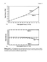
Figure 6.16 illustrates the effect
of
increasing the rotor weight on the
whirl. The results show that increasing the rotor weight from 45.5kg to
142
kg
increases the speed for the instability threshold.
It
also significantly
reduces the whirl amplitude.
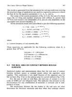
Changes
in
the whirl conditions can be seen in Fig. 6.17, when the
bearing clearance is changed from 0.0063in. to 0.01 in. (0.016 to
Design
of
Fluid
Film
Bearings
181
0.03
, ,
I I
-0.03
-0.03
-0.02
-0.01
0.00
0.01

0.02
0.03
XI0
7
,,,,,,,,,,,,*,,,,,,f
6-
5-
E-
04-
E:
-
z:
u3-
5-
f:
:
2-
1-
0.56
0.57
0.58
0.59
0.60
Eccentricity
Ratio,
E
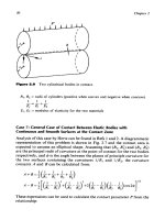
Figure
6.12
(a) Synchronous whirl for balanced
rotor

at
1750
rpm. (b)
Eccentricity-time plot for unbalanced
rotor
at
1750
rpm.
182
Chapter
6
-0.2
1
s
0
<
0.0
0.1
0.2
0.3
0.4
0.5
Ecoontrlcity
Ratio,
E
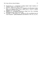
Figure
6.13
(a) Nonsynchronous whirl
for
balanced

rotor
at
5500
rpm.
(b)
Eccentricity-time plot
for
unbalanced
rotor
at
5500
rpm.
Design
of
Fluid Film Bearings
1.01
. .
,
.
.
.
.
,
.
*.
.I.
- - -
1
0.5
-1.0

-0.5
0.0 0.5
1
.o
xlo
15
IR
f
'0
10
L
a
5
183
0
0.0
0.2 0.4 0.6
0.8
1
.o
Eccentricity
Ratio,
6
Figure
6.14
(a) Whirl
of
unbalanced
rotor
at sleeve contact condition

(6100
rpm). (b) Eccentricity-time plot for unbalanced
rotor
at
6100
rpm.
184
Chapter
6
.7

Y
n
n
n
n
c) c)
A A
n
n
n
n
c)
Y
n
"
.8
Y
Y
Y

3,-
.c
n
1
I
I
I
I
I
O.Oo0
0.001
0.m
0.m
0.004
0.005
0.006
0.007
WhS)
kw
l~l~l~l~l'l-l
O.oo00 O.ooo5
0.0010 0.0015
O.Oa20
0.0025
O.Oo30
5ooo
P
Y
0
0

v)
8
(b)
0
O.Oo0
0.001
0.002
0.003
0.004
0.005
0.008
0.007
mr
(Ibm-8q
~-I-I.I-I-I-I
O.OMx1
O.oo(#
0.0010 0.0015
0.0020
0.0025
O.Oo30
kg-8*
Figure
6.1
5
(b)
Spectrum
of
transient peak eccentricity for unbalanced rotor.
(a) Spectrum

of
steady-state peak eccentricity for unbalanced
rotor.
Design
of
Fluid Film Bearings
185
w
0.4
-
w=
142
ko
0.2
-
-

W
-
46.6
kg
nu
=
0.000227
kgd
0
SbadyS1.1.EfmntrMyfor8.kncrdRotor
0.0
1.1.1.1.1.1.
0

1000
2000
3000
4000
5000
6000
7000
Figure
6.16
(a) Effect
of
rotor
weight on steady-state peak eccentricity for dif-
ferent unbalanced magnitudes.
(b)
Effects
of
rotor weight on amplitude of whirl
(mr
=
0.000227
kg-sec2).
186
Chapter
6
1
.o
0.8
0.6
w

0.4
0.2
0.0
Speed
(vm)
Figure
6.1
7
(a) Effect
of
clearance on steady-state peak eccentricity
for
different
unbalanced magnitudes.
(b)
Effect
of
clearance on amplitude
of
whirl
(mv
=
0.000227 kg-sec2).
Design
of
Fluid Film Bearings
187
0.0254 cm). Figure 6.17a shows that increasing the clearance causes a reduc-
tion in the instability threshold. Figure 6.17b on the other hand, shows little
effect on the actual whirl orbit amplitude due to the clearance change with

0.000227 kg-sec2 unbalance.
Two opposite effects of changing the average film temperature are
shown in Fig. 6.18. In the first example, with
W
=
lOOlb (45.5 kg),
C
=
0.0063 in.
(0.0
16 cm), and
mr
=
0.005 lb-sec2 (0.000227 kg-sec2),
increasing the average film temperature from 373°C to 94°C resulted in a
considerable reduction in the threshold speed, as well as an increase in the
whirl amplitude (Fig. 6.18a). On the other hand, the second example,
W
=
1000 lbf
=
455 kg and
C
=
0.016 cm, shows that considerable reduc-
tions in the whirl amplitude resulted from the same increase in the average
film temperature (Fig. 6.18b).
The case of
a
rigid rotor on an isoviscous film considered in this illus-

tration provided a relatively simple model to approximately investigate the
effect of rotor unbalance and film properties on the rotor whirl.
The developed response spectrum shown in Fig. 6.15a gives a complete
view of the nature of the rotor whirl as affected by the speed and the
unbalance magnitude. Of particular interest is the existence of a rotational
speed for any particular unbalance where the peak eccentricity is minimal.
Nonsynchronous whirl, with increasing amplitudes and eventual instability
or rotor sleeve contact, occurs as the speed is increased beyond that condi-
tion. It should be noted here that results associated with large whirl ampli-
tudes and those near bearing walls represent qualitative trends rather than
accurate evaluation of the whirl in view of the assumptions made.
Investigation of the influence of system parameters on whirl for the
considered cases showed, as expected, that improved rotor performance
can be attained by increasing the load and reducing the clearance.
Increasing the average film temperature showed that an increase
or
a reduc-
tion in the whirl amplitude may occur depending on the particular system
parameters.
Although a relatively simple model is used in this study, the technique
can be readily adapted to the analysis of more complex rotor systems and
film properties.
6.2
DESIGN
SYSTEMS
6.2.1
This is an illustration of graph-aided design for journal bearings. The
graphs are constructed in such a manner as to enable the designers to
Procedure Based on Design Graphs
188

1
.o
0.8
0.6
w
0.4
0.2
0.0
Chapter
6
Figure
6.18
(b)
W
=
455
kg.
Effect
of
average film temperature
on
rotor whirl: (a)
W
=
45.5
kg;
Design
of
Fluid
Film

Bearings
189
select the bearing parameters, which meet their objective with a minimum
of calculations.
In constructing the graphs, the main parameters influencing the bearing
behavior were divided into two groups.
The first deals with the bearing geometry
(L,
D,
R,
C),
load
W,
and
speed
N.
The second deals with the oil, and its temperature-viscosity char-
acteristics. Because many types of oil can be used in the same bearing, the
basic approach in the design graphs given here is to construct separate
graphs for the different bearings and oils.
The bearing graphs represent a plot
of
temperature rise,
Af,
versus
average viscosity for a bearing with a known characteristic number,
K
=
(R/C)2N,
length-to-diameter ratio,

t/D,
and average pressure
P.
They are constructed by assuming the average viscosity, calculating the
Sommerfeld number and the corresponding
A
T.
Such plots are based on the numerical results of Raymondi and Boyd
[24]
and are shown in Figs
6.19-6.22
for average pressure values of
100,
9E-6
8E-6
7E-6
6E-6
5E-6
n
4E-6
f
a
3E-6
3.
2E-6
1
E-6
P=lOOpsi
___
Ud

I
1.0

Ud
0.5

Ud
=
0.25
0
20 40
60
80
100 120 140 160 180 200 220 240 260 280
AT
(OF)
Figure
6.19
Bearing chart for
P
=
1oOpsi.
9E-6
8E-6
7E-6
6E-6
5E-6
a
3E-6
2E-6

1
E-6
Ud
m
0.2s
ud
10.5

P
=
SO0
p.1
Udml.O
0
20
40
60
80
100 120 140 160 180 200 220 240 260 280
AT
(OF)
Figure
6.20
Bearing chart for
P
=
500
psi.
9E-6
8E-6

7E-6
6E-6
5E-6
2E-6
1
E-6
0
20
40
60
80
100 120
140
160
180
200
220
240
260
280
AT
(OF)
Figure
6-21
Bearing chart
for
P
=
1OOOpsi.
Design

of
Fluid Film Bearings
191
9E-6
8E-6
-
7E-6
-
6E-6
-
5E-6
-
n
4E-6
-
s?
3E6
-
3.
2E-6
-
1
E6
0
20
40
60
80
100 120
140

160 180 200 220 240 260 280
AT
(OF)
Figure
6.22
Bearing
chart
for
P
=
2000psi.
500,
1000,
and
2000
psi, respectively. The length-to-diameter ratios
LID
considered are
0.25,
0.50,
and 1.0.
The graphs for the lubricants represent the change of average viscosity
with temperature rise for any particular initial temperature. Figures
6.23-
6.25
represent such plots for
SAE
10,
20,
and

30
oils, respectively. These
graphs give a convenient means of analysis, as
well
as the design of bearings,
as explained in the following section.
Analysis
Procedure
For a bearing with a given geometry, load, and speed,
a
characteristic
number,
K
=
(R/C)2N,
can be readily calculated.
As
can be seen from
Eq. (6.8),
this number represents the Sommerfeld number for a particular
value
of
viscosity and average pressure. That is:
K
=
S(F)
9E-6
8E-6
7E-6
6E-6

5E-6
4E-6
n
r)
5
3E-6
e
Y
=L
2E-6
1 E-6
SAE
10
t,
=
40
-
170
OF
0
20 40 60
80
100 120 140 160 180 200
220
240 260
280
AT
(OF)
Figure
6.23

SAE
10
oil
chart.
9E-6
8E-6
7E-6
6E-6
5E-6
4E-6
n
(D
3E-6
t
U
3.
2E-6
1 E-6
0
20
40
60 80 100 120 140
160
180 200
220
240 260 280
AT
(OF)
Figure
6.24

SAE
20
oil
chart.
Design
of
Fluid Film Bearings
I93
9E-6
8E-6
7E-6
6E-6
5E-6
4E-6
3.
2E-6
1
E-6
0
20 40 60
80
100
120
140 160
180
200
220
240 260 280
AT
(OF)

Figure
6.25
SAE
30
oil
chart.
The bearing graph (which represents the relationship between viscosity,
p,
versus temperature rise,
At,
for
the
particular value of
K,
LID,
and
P),
can be
readily plotted on a transparent sheet by interpolation from Figs 6.9-6.12.
Given the type of oil and its inlet temperature, the oil graph (which represents
average viscosity versus temperature rise for the oil), is also plotted on the
same sheet from Figs 6.23-6.25. Intersection of the two curves as can be seen
in the example illustrated in Fig.
6.26,
gives the temperature rise in the bear-
ing and the corresponding average viscosity,
p.
The Sommerfeld number for
the bearing is then calculated from
S

=
Kp/P.
Consequently, all the behavioral characteristics of the bearing can be
read from Figs 6.3-6.8
or
calculated from the given bearing performance
equations, which are based on the curve fitting
of
these figures.
illustrative
Example
The use of the bearing design graphs
is
illustrated by the following example.
It is assumed that a shaft 2 in. in diameter, carrying a radial load of 2000 lb
194
Chapter
6
9x1
o8
8x1
O8
7x1
O8
6x1
0"
5x1
0"
4x10"
3x106

n
*
B
2x1
o8
1
OS
0
20 40 60 80
100
120 140 160
180
200
220 240 260 280
AT
(OF)
Figure
6.26
Bearing design chart: application for clearance selection.
at 10,000rpm is symmetrically supported by two bearings, each of length
1
.O
in. The lubricating oil is
SAE
No.
10 with an inlet temprature of 150°F.
The objective
is
to select a value for the radial clearance,
C,

which minimizes
both the oil
flow and temperature rise. Because these are conflicting
objec-
tives, a weighting factor,
k,
has
to
be specified to describe their relative
importance for a particular bearing application. The design criterion can
therefore be formulated as:
Find
C,
which minimizes
U
=
At
+
kQ
(6.15)
where
At
=
temperature rise (OF)
Q
=
oil
flow
(in.3/sec)
Values of

k
=
2,
5,
and
7
are considered to illustrate the influence of the
weighting factor on the final design.
The average pressure and the length-to-diameter ratio are first calcu-
lated as:
Design
of
Fluid Film Bearings
195
L
LD
1x2
D
-
5oOpsi
and
-
=
0.5
p=-=
w
2000/2
Arbitrary values for the design parameter,
C
are assumed and the corre-

sponding bearing parameter,
k,
is calculated in each case. For example, if
C
is selected equal to 0.006in., the corresponding parameter is
=
(+=
(&)
*
(7)
107000
=4.63
x
106
The bearing performance curve, corresponding to this value of
k
for
P
=
5OOpsi and
LID
=
0.5, can be interpolated from Fig. 6.21 as plotted
in Fig. 6.26. The oil characteristic curve for SAE 10 for the 150°F inlet
temperature is also traced from Fig. 6.23 as shown in Fig.
6.2.
The inter-
section of the two curves yields the following values for the temperature rise
and average viscosity:
Al

=
15°F
and
p
=
1.53
x
10-6
reyn.
The Sommerfeld number is then calculated:
kp
P
500
(4.63
x
106)(1.53
x
10-6)
S=-=
The quantity of oil
flow,
Q,
is readily found from Fig.
6.5
as
Q
=
5.8
RNCL
=

5.8 ir~.~/sec
The merit value is calculated from
Eq.
(6.15) for the given weighting factor,
k.
The process is repeated for different selections of the clearance
(0.003
in.
and
0.0
12
in. are tried in this example).
The
results are listed in Table 6.1 and
plotted in Fig. 6.27.
Table
6.1
Numerical Results
for Bearing Design
U
Q
C
CL
(reyn)
C
At
(“F)
(in.3/sec)
k
=

2
k
=
5
k
=
7
0.003 1.22
x
10-6
0.0454
38 2.81 43.62
52.05 57.67
0.006
1.53
x
10-6
0.0142
15
5.81
26.6
44
55.6
0.012 1.61
x
10-6
0.00375 8 12.00
32 68
92
196

Chapter
6
O.OO0
0.002
0.004
0.006 0.008
0.010
0.012 0.014
Clearance,
C
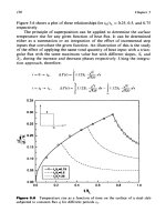
Figure 6.27
Selection
of
optimum
clearance for the difference objectives.
The optimum clearances can be deduced from the figure for the different
values of the weighting factor
k
as:
k
=
2:
C*
=
0.005in.
k
=
5:
C*
=

0.006in.
k
=
7:
C*
=
0.007in.
6.2.2
Automated
Design
System
This section presents an automated system for the selection of the main
design parameters
to
optimize the performance of the hydrodynamic bear-
ing. In spite of the wealth of literature on the analysis of these bearings, the
selection of design parameters in the past has relied heavily on empirical
guides. Empiricism was necessary because of complexity of the interaction
between the different parameters which govern the behavior of such bear-
ings. The analytical relationships describing the bearing performance are
Design
of
Fluid Film Bearings
197
generally based on Reynolds’ equation and are, in most cases, numerical
solutions of the equation with certain assumptions and approximations.
In this section, the curve-fitted numerical solutions, given in Sections
6.1.3 and 6.1.4, are utilized in a design system that rationally selects the
significant parameters of a bearing to optimally satisfy the designer’s objec-
tive within the constraints imposed on the design.

A
full journal bearing to
operating at a constant speed and supporting a known constant load is
considered. The procedure is extended to cover the selection of an optimum
bearing for applications where the load and speed may vary from time to
time within given bounds.
System Parameters
The main independent parameters for the problem under consideration are
(D,
L,
C),
p,
and
(W,
N).
These parameters, as grouped, describe the bear-
ing geometry, oil characteristics, and load specifications, respectively.
In
formulating the problem, it will be assumed that
D,
N,
W
are given inputs
for the bearing design. The design parameters are therefore
LID,
C,
p.
The
constraints on the design are:
The first five of these inequality constraints represent the limit on the oil film

thickness, temperature rise, maximum allowable pressure, minimum oil visc-
osity, and bearing length. These limits are dictated by the quality of machin-
ing, the characteristics
of
the material-lubricant pair, and the available
space. The sixth constraint describes a condition for bearing stability, as
described in Fig. 6.8.
The Governing Equations
The equations governing the behavior
of
the bearing in this study are devel-
oped by curve fitting from Raimondi and Boyd’s numerical solution to
Reynolds’ equation, Eq. (6.1). These equations, which are given in Section
6.1.3, allow the calculation of the temperature rise, minimum oil film thick-
ness, maximum oil film pressure, oil
flow,
frictional
loss,
and
so
forth. The
I98
Chapter
6
curve-fitted equations for the stability analysis by Lund and Saibel, given in
Section
6.1.4,
provide a simplified mathematical relationship for the onset of
instability constraint.
Design Criterion

The selection of an optimum solution requires the development of a design
criterion, which accurately describes the designer’s objective. The topogra-
phy of this criterion and its interaction with the boundaries of the design
domain (constraint surfaces), have a significant effect on the efficiency and
success of the search. In the problem of bearing design, many decision
criterion can be envisioned. Some of these are: minimizing the maximum
temperature rise of the bearing, minimizing the quantity of oil flow required
for adequate lubrication, minimizing the frictional loss, and
so
forth. The
objective may also be composed of a multitude of the previously mentioned
factors, and weighing their relative importance requires skilled judgement by
the individual designer.
Search Method
In formulating the problem for automated design, the following factors are
considered in developing a search strategy:
(I)
the nature of the objective
function,
(2)
the design domain and behavior of the constraints,
(3)
the
sensitivity
of
the objective function to the individual changes in the decision
parameters, and
(4)
the inclusion of a preset criterion for search effectiveness
and convergence.

A block diagram describing the search is shown in Fig.
(6.28).
Arbitrary
values of the design parameters within their given constraints are the entry
point
to
the system. These values need not satisfy the functional constraints.
The first phase of the search deals with guidance of the entry point into the
feasible region. In this phase, incremental viscosity changes, of the order of
10%,
and clearance changes, on the order of
0.001
in. per inch radius,
proved to be adequate. When the stability constraint is violated, a feasible
point may be located by dropping the length-to-diameter ratio to its lower
limit, and simultaneously halving the viscosity and the clearance. To avoid
looping in this phase, a counter can be set to limit the number of iterations.
If a feasible point can not be successfully located, the designer can readjust
the entry point according to the experience gained from the performed
computations. When a feasible point in the design domain is located, the
gradient search is initiated according to:
Design
of
Fluid Film Bearings
199
I
1
Inputs
W,
R,

N.
C.
P,
Ud
(within
side
consUaints)
I
StaltGradiiSearch
+
I
1
Wmin
Feasible
Region
(a)
violated
satisfedory
Point
Locatrn
Figure
6.28
(a) Search method
flow
diagram
1.
(b)
Search method
flow
diagram

2.
200
P,+I
=
Pn
-
Chapter
6
where
n,,
nc,
and
nL
=
scale factors
If
p
is taken as the reference parameter, these factors can be determined
from:
n,
= =
I
nc7
=
1:l
=
order of
103
nL
=

141
=
order of
10s
The control of the step size is exercised by including a provision for chan-
ging
A,,
in the computational logic. One way to accomplish this is to require
a specified percentage change in one of the parameters and to set upper
limits on the incremental changes in the other parameters, thus offering a
safeguard against the overshooting of the gradient.
If
the new point fails to
produce an improvement in merit, the step size is halved several times and
the process repeated, if necessary, in the reverse direction
of
the gradient.
Nonimproving merit along both directions indicates an optimum at the base
point. If the new point is found to be of higher merit, yet violating the
functional constraints, the univariate search is activated. In this phase, the
parameters are allowed to undergo incremental changes
of
10%
over a
range
of
f90%
for the viscosity and
LID
ratio, and

5%
over a range of
45%
for the clearance. The first check, made after each iteration, is on the
functional constraints (maximum temperature, maximum pressure, mini-
mum film thickness and stability). The success of returning to a feasible
point is followed by comparing its merit value to that of the last base
point.
A
higher merit produces a new base point, while failure to reach a
feasible point with improved merit indicates an optimum at the last feasible
location. An illustration of the design region, and search progression is
given in
Fig.
6.29
for a two parameter problem where
LID
is assumed
constant.
Design
of
Fluid
Film
Bearings
20
I
Clearance
Figure
6.29
Design region and search progression for the two-parameter pro-

blem
(LID
=
constant).
Numerical
Examples
Two
common bearing applications are considered
to
illustrate the design
procedure.
Design
of
Bearings
for
Constant
Load
and Speed Condition
The inputs are taken as:
W
=
2000, 1000,500,2501b, respectively
N
=
16.66,33.33,83.33, 16666,250,333.33 rps,
respectively
D
=
2in.
The constraints are:

hmin
=
5
x
10-’in.
tmin
,,
=
300°F
=
maximum allowable temperature
Pm,,
=
30,000
lb/in?
=
maximum allowable pressure
202
L
-=
1.0
Drnax
Chapter
6
-
0.25
L

Dmin
pmin

=
1
x
10-’
reyn
It is assumed that the design objective is to minimize both the oil supply to
the bearing and the oil film temperature rise with a relative merit factor of
5
:
1, respectively. this may
be
stated as:
Minimize
U
=
Af
+
5Q
subject to the given constraints
Results. The optimum bearing parameters for the considered exam-
ples are illustrated in Figs
6.30-6.32.
These parameters are unique combi-
nations and are obtained irrespective of the starting point. Figures
6.33-
6.37
show the corresponding operative characteristics.
It can be seen from the results that the optimum clearances are higher
for high loads and low speeds to satisfy the minimum film thickness require-
ment. Figure

6.31
shows that relatively high lubricant viscosity is relied
0
W
=
250
0
W
=
500
0
w
=
2000
.008
m
A
w
f
1000
0
c
W
0
.006
z
2
.007

a

a
a
.005
0
J
5
.004
a
a
a
.003
I
I
1
I
I
5000
lop00
15,000
20,000
SPEED
RPM
Figure
6.30
Optimum
clearance.
Design
of
Fluid
Film

Bearings
D
W.500
-
A
w
=
1000
ow=2ooo
-
-
-
A
203
SPEED RPM
Figure
6.51
Optimum values
of
average viscosity.
0
F
5
0.45
0.40
z
S
0.35
c3
'

0.30
I
c
(3
z
W
A
2
0.50
II
1
1
1
I
-
W
=
250
5000
10,000
15,000
20mO
SPEED
RPM
Figure
6.32
Optimum length/diameter ratio.
204
II
I

1
I
1
W
=
250
A
W
=
1000
0
w
=
2000
-
0
W=500
-
-
-
-
I1
I
1
I
I
Chapter
6
5000
10,000

15,000
20,000
SPEED RPM
Figure
6.33
Temperature rise in optimum bearings.
5
20
2
w
l5
a
2
10
W
a
3
I-
W
Q
r
W
k5
Figure
6.34
Oil requirement for optimum bearings.