Friction and Lubrication in Mechanical Design Episode 1 Part 10 pptx

Design
of
Fluid Film Bearings
205
Nc
30,000
e

\
W
U
3
v)
v)
E
20,000
a
r
3
H
X
z
-
a
10,000
0
-
W
=
250
0

w
=
500
A
W
=
1000
0
w
=
2000
JI
I
I
I
I
I
5000
10,000
I5,OOO
20,000
SPEED
RPM
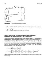
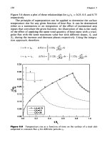
Figure
6.35
Maximum
oil
pressure in optimum bearings.
W
=

250
0
W
=
500
A
W
=
1000
$
0.6
5000
10,000
15,000
20,000
SPEED
RPM
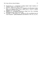
Figure
6.36
Frictional
loss.
206
60
50
>
p
P
30
W
r

20
10
11
I
I
1
1
Chapter
6
5000
10,000
15,000
20,000
SPEED
RPM
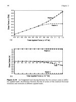
Figure
6.37
Merit
value
for
optimum designs.
upon at low speeds to maintain the required film thickness. As the speed
increases and the journal eccentricity becomes smaller, the optimal viscos-
ities drop in order to satisfy the stability criterion. This trend continues as
speed increases until the lower limit set on the viscosity is reached.
Although longer bearings may have higher merit values (according to
the design criterion under consideration), the drop in the optimum
LID
ratio with increasing speed is primarily induced by stability requirements.
Figure 6.33 shows an increase of temperature rise

of
the optimum bear-
ing with increased speeds and loads. A similar trend can be seen in Fig. 6.34
for the quantity of oil to be fed to the bearing. The maximum oil film
pressure, Fig. 6.35, generally increases with increasing load at any speed.
For any particular load, the changes in maximum film pressure with speed
are influenced by the corresponding changes in radial clearance.
The frictional power
loss
(Fig. 6.36) and the value
of
the objective
function (Fig. 6.37) increase with increased loads and speeds.
The effect of the weighting factor,
k
on the final design is illustrated for
the case where
W
=
10001b, and
N
=
166.66 rps. The results are given in
Table 6.2.
It
can be seen that by taking
k
=
1,
5,

and
10,
respectively, the tempera-
ture rise for the optimum bearings are 3.77,
11
.O,
and 14.44"F, respectively.
Design
of
Fluid
Film
Bearings
20
7
Table
6.2
Effect of Weighting Factor,
k,
on the Optimum Design
(W
=
100
lb,
N
=
166.6rps)
Weighing
Q
(in.'/
ha,

factor
k
P
C
LID
Af
(OF)
sec)
(psi)
HP
loss
1 1
10-~
3.4
10-~
0.36
3.77 4.88 7600 0.147
5
1
x
10-7 2.55 x 10-3 0.325 11.00 2.15
8500
0.175
10
1
x
10-7
1.5
x
10-3

0.313
14.44 1.67
6500
0.185
The corresponding values of the oil flow are
4.88,2.15,
and 1.67 in.3/sec. It is
interesting to note this change in objective produced no change in the
required average viscosity since it is already at its lower limit.
A
small
change is necessary however, in the length-to-diameter ratio but the most
significant change is in the required clearance.
Bearings Operating Within a Range
of
Specified Loads and Speeds
The previous design system
is
extended
so
that the optimum parameters, for
a bearing operating with equal frequency within a given range
of
loads and
speeds, may be automatically obtained.
In this case, the region under consideration is divided into an array
of
points, each representing a particular load and speed.
A
search procedure,

similar to that previously mentioned, is adopted. In this case, however, the
feasibility
of
the design at each step is checked for all points in the array.
The merit values are also calculated at
all
points, and the lowest
of
these
values is taken to represent the merit rating of the bearing.
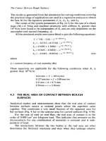
Results.
Optimum bearing parameters corresponding to several
load-speed regions are given in Table 6.3. The input data, constraints,
and design criterion are the same
as
in the previous examples. The regions
considered are illustrated in Fig.
6.38.
Some
of
the results shown in the
table are obtained for the case where only the corners of the regions (i.e.,
a
point array) are considered.
To
investigate the effect of grid size on the
design, regions
2
and
5

are each divided into a
3
x
4
grid. The results, as
shown in the table, do not appreciably change with the change of grid
size. In all the studied cases, the point of lowest merit is found to be that
when both load and speed are highest.
Figure 6.39 shows a comparison of the results from the regional search
and those obtained for an optimum bearing designed for the maximum load
and speed in region
2.
The latter, as expected, shows a higher merit for the
load and speed for which it is selected, but its operation is constrained at
other parts
of
the considered region
as
indicated by the asterisk marker.
208
Chapter
6
Table
6.3
Optimum Bearing Parameters and Corresponding Operative Characteristics;
V
=
5Q
+
At

~~~
~
~
~
~
Max.
Max. Max. Max. Qfriction Max.
Ar
in
P,,,
in Min.
ho
in
loss
in merit
Region Load range Speed range Grid region region in region region region value in
no.
(W
(rpm) points (reyn)
C
(in.)
LID
(OF)
(lb/in.2) (in.) (in./sec) (hp) region
1
500-1,000
1,000-5,000
2
x
2

1.3
x
10-7
1.90
x
lO-’
0.990
8.0
1,187 5.06
x
10-5
1.519
0.115 15.73
2
1,000-2,000 1,000-5,000 2
x
2
3.0
x
10-7
2.55
x
10-3 0.990
12.5
2,607 5.00
x
10-5 2.100
0.234 23.03
2
1,000-2,000

1,000-5,000
3
x
4
3.1
x
10-7 2.64
x
10-’
0.998
12.3
2,592 5.07
x
10-5 2.180 0.237 23.20
3
500-2,000
5,000-10,000 2
x
2 6.2
x
10-7 5.90
x
10-’ 0.280 17.1 28,380 5.04
x
10-5
4.500 0.430 39.80
4 1,000-2,OOO 10,000-20,000
2
x
2

3.0
x
10-7
4.07
x
10-3 0.275 27.6
24,750
5.14
x
10-5 6.000 0.968 57.70
5
500-1,000 10,000-20,000
2
x
2
1.14
x
10-7 2.95
x
10-3
0.300
17.7 9,633 5.00
x
lO-’
4.500
0.484 40.29
5
500-1,000
10,000-20,000
3

x
4 1.4
x
10-7 3.00
x
10-’ 0.275
19.6
10,860 5.16
x
lO-’
4.450 0.523 41.80
Design
of
Fluid Film Bearings
5.09
5.89.
209
8.8
15.5.
I85
9.76.
16.4.
19.45.
Y
2000
U)
E
a
0
3

1000
1000
5000
10,000
20,000
500
SPEED
RPM
Figure
6.38
Considered load and speed regions.
10.2
17.7.
21.1.
11.8
ui
5.55.
9.5
16.7.
0
1500
10.8.
18.1.
21.4.
a
6.6
-
I
a
3

Figure
6.39
Comparison
of
designs obtained by regional search and those
obtained
for
the
maximum
condition
of
load
and speed (Region
2).
6.3
THEROMODYNAMIC
EFFECTS
ON
BEARING
PERFORMANCE
In the classical hydrodynamic theory presented by ReynoIds
[I],
an isovis-
cous film
is
assumed. This assumption
is
widely used in bearing design,
because accounting for the effects of temperature variations along the lubri-
cant film and across its thickness would significantly complicate the analysis.

Many experimental observations, however, show that the isoviscous
hydrodynamic theory, alone, does not account
for
the load-carrying capa-
city and the temperature rise in the fluid film. McKee and McKee
[15],
in a
210
Chapter
6
series of experiments, observed that under conditions of high speed, the
viscosity diminished to a point where the product
pN
remained constant.
Fogg
[
161
found that a parallel-surface thrust bearing can carry higher loads
than those predicted by the hydrodynamic theory. His observation, known
as the Fogg effect, is explained by the concept of the “thermal wedge,”
where the expansion of the fluid as
it
heats up develops additional load-
carrying capacity. Shaw
[
171,
Boussages and Casacci
[
181,
Osterle et al.

[
191,
and Ulukan
[20]
are among the investigators of thermal effects in fluid film
lubrication. Cameron
[2
11,
in his experiments with rotating disks, suggested
that a hydrodynamic pressure
is
created in the film between the disks arising
from the variation of viscosity across the thickness of the film. This variation
is generally referred to as the “Cameron effect.” Experiments by Cole
[22]
on temperature effects in journal bearings indicated that at high speeds,
severe temperature gradients are set up, both across the film because of
heat removal by conduction and in the plane of relative motion because
of
convective heat transfer from
oil
flow. He accordingly suggested that
constant viscosity theory under such conditions should be applied with
caution. Hunter and Zienkeiwicz
[23]
presented a theoretical study of the
heat-energy balance of bearings and compared their findings with Cole’s
results. They concluded that the effect
of
temperature, and consequently,

viscosity variations across the film in a journal bearing is by no means
negligible. Thus pressures were lower than those obtained from a solution
which takes into account the viscosity variation along the length of the film
only, and the decrease in pressure is more pronounced in the case of non-
conducting boundaries than
if
the boundaries were kept at the lubricant
inlet temperature. Their attempts to predict an effective mean viscosity,
which would lead to a correct estimate of pressure, were hampered by the
fact that such an average value would be clearly a function of the boundary
temperature as well as the mean temperature of the oil leaving the bearing.
Dowson and March
[24]
carried out a two-dimensional thermodynamic
analysis of journal bearings to include variation of lubricant properties
along and across the film. They presented temperature contours in the
film, as well as a reasonable estimate of the shaft and bush temperatures.
It was observed during experimental investigations of the pressure dis-
tribution in the fluid film developed by rotating an externally supported
journal in a sleeve at a predetermined eccentricity that
[25-281:
1.
Both the circumferential and axial patterns of pressure distribu-
tion normalized to the maximum pressure (Fig.
6.40)
are identical
to those predicted by the isoviscous hydrodynamic theory (Refs
2-4
for example).
Design

of
Fluid Film Bearings
21
I
.
w
3
v)
v)
w
a
a:
+o
Experimentol
0.
0.25
111
I1111
I
20
40
60
80
I00
I20
140
160
18
IL
CIRCUMFERENTIAL

LOCATION
8"
'1!
8
I
mid-
plo
ne
AXIAL
LOCATION
in.
Figure
6.40
Normalized pressure distribution. (From
Ref.
25.)
2.
For any particular eccentricity, oil, and inlet temperature, the
magnitude
of
the peak pressure (or the average pressure) in the-
film is approximately proportional to the square root of the rota-
tional speed
of
the
journal
rather than the approximately linear
proportionality predicted by the isoviscous theory (Fig.
6.4
1).

For
any
particular eccentricity, oil, and inlet temperature, there
exists a speed
N*
where the isoviscous theory predicts the same
magnitude
of
maximum pressure,
PkaX
(and consequently, aver-
age pressure
P:,)
as that measured experimentally (Fig.
6.41).
For a given film geometry (fixed eccentricity), oil, and speed, the
variation
of
the maximum pressure (and consequently the aver-
age pressure) with inlet temperature is different than that pre-
3.
4.
212
Chapter
6
-1
a/-
/
b/
,C

=.015
/
>At
3U
__
n-
*
128.F
/
/
-
Expcrimenfol
-
-
Hydrodynomic
Liroviscous
1
/
I
1
I
1
1
1
I
'/
'
175
L
*

I
"
,
D
2'
150
t
zc
,
I
1
-1-
A
-
SPEED,
RPM
Figure
6.41
27.)
Pressure-speed relationship for fixed geometry bearing. (From Ref.
dicted by the isoviscous theory. Only at the
O*
point can the
isoviscous theory predict the film pressures.
For any particular eccentricity, speed, and oil, the
O*
condition
(where the experimental and predicted isoviscous bearing perfor-
mances are identical) can be determined according to the
follow-

ing empirical procedure (see Fig.
6.42):
5.
p,*-
N=N*
\
\,Hydrodynamic
(
isoviscous
1
To
Figure
6.42
(E
=
constant).
Procedure for determination of the thermohydrodynamic
o*
point
Design
of
Fluid Film
Bearings
213
Construct the curve relating the average pressure,
P,,
to the
average film temperature,
Tu,
based on the isoviscous theory.

Since
E
is fixed and
LID
is known, the isoviscous Sommerfeld
number
Siso
is constant and can be readily determined by the
isoviscous theory. Therefore
S,,
=
constant
=
-
-
($
and consequently, for any speed
N,
a curve can be plotted to
relate
P,
and
Tu
(which for a given oil defines the average
viscosity
p,).
The
O*
condition is found empirically to be the point on that
curve where the slope of the tangent is:

dPa
V
tan/?=
-
dTa
K
where
V
=
volume
of
the
oil
drawn into the clearance space
in cubic inches
per
revolution
K
=
constant which is found empirically (based
on
the
experimental results from Refs
25-32
as detailed in
Ref.
33)
to
be
a

function
of
(R/C)
as
plotted
in
Fig.
6.43
K
(%OF)
Figure
6.43
The empirical factor
k.
214
Chapter
6
(c) The temperature rise
AT*
at the
O*
condition can be readily
determined based on the isoviscous theory. Consequently,
the oil inlet temperature corresponding to this condition
can be calculated from:
AT*
2
Ti
=
T'

-
-
For a given eccentricity, oil, and inlet temperature,
Ti,
the
pressure-speed relationship can be empirically expressed as:
(6.16a)
Since the pressure distribution as predicted by the isoviscous
theory remains the same (Fig.
6.40),
therefore:
(6.16b)
This relationship is illustrated in Fig.
6.44
and compared to
the corresponding pressure-speed relationship predicted by
isoviscous considerations for the same conditions.
6.3.1
Basic Empirical Relationships
The objective of the following is to develop, based on experimental findings,
a modified Sommerfeld number
S*
(and consequently, an effective average
W
K
3
v)
v)
w
K

Q
W
SPED
N
Figure
6.44
Pressure-speed relationship for
a
fixed geometry bearing.
Design
of
Fluid Film Bearings
215
viscosity) for any bearing, which accounts for the thermohydrodynamic
behavior of the film and can be directly used instead of
S
to evaluate the
performance characteristics for any operating condition, using existing iso-
viscous analysis and data.
Based on isoviscous hydrodynamic considerations, the Sommerfeld
number,
S,,
for a bearing with a given film geometry is independent
of
speed, oil, and inlet temperature. Consequently, the relationship between
the pressure,
P,,
speed,
N,
and average viscosity,

p,,
is governed by the
condition:
Now defining
S*
at the
O*
condition as
(6.17)
(6.18)
For the same
E,
Siso
=
S*,
from which:
From
Eq.
(6.18),
which is based on the empirical observation for a given
film
geometry, oil, and inlet temperature,
Ti:
N
PO
=
average pressure
in
the film with inlet temperature
Ti

=
V
(6.20)
where
QIRNCL
is
calculated based
on
isoviscous considerations from
Sis,
and
LID.
From
Eq.
(6.19):
216
Chapter
6
Assuming the following viscosity-temperature relationship:
p
=
where
po,
8,
and
6
are constants for the given oil (Table
6.4)
and
T

is the
temperature of the oil, the isothermal Sommerfeld number
(S)j.Fo
for the film
at a speed
N
and average temperature
To
can be written as:
from which:
and by differentiation:
(6.21)
from which
7‘:
can be evaluated by iteration. Consequently
(AT)*
can be
evaluated by isoviscous considerations and the corresponding
Tj
can be
calculated from:
Table
6.4
Oil
Constants
SAE 10 1.18
x
10-5
2.18
x

10-6
1.58
x
10-8
1
157.5
SAE
20
1.95
x
10-’
3.15
x
10-6
1.36
x
10-*
1271.6
SAE 30 3.35
x
10-’
4.60
x
10-6
1.41
x
10-’ 1360.9
SAE 40
5.50
x

10-’
6.40
x
10-6 1.21
x
10-*
1474.4
SAE
50
9.50
x
10-5
1.05
x
10-5
1.70
x
10-8
1509.6
SAE 60 1.42
x
10-s
1.45
x
10-5
1.87
x
10-*
1564.0
Viscosity at any temperature

T(”F)
is
given by
p(T)
=
poeh’(T+N),
where
8
=
95°F
and
po
=
lubricant relative viscosity.
Design
of
Fluid
Film
Bearings
21
7
The thermohydrodynamic pressure-speed relationship for the particular
film geometry is, according to
Eq.
(6.16):
If
it
can be assumed that
T,*
is known or can be approximately estimated for

a particular oil and film geometry, the corresponding
N*
can be computed
directly from Eq.
(6.21)
as:
This equation can be reduced to give:
(6.22)
which can be readily determined by isoviscous considerations for a given
E,
oil,
LID,
C/R,
and
T,.
6.3.2
Prediction
of
Bearing Performance
In a practical situation, the following bearing parameters are usually given:
load
W,
diameter
D,
length
L,
radial clearance
C,
journal speed
N,

and oil
and inlet temperature
Tj.
In this section, two empirical procedures will be given for determining a
modified Sommerfeld number
S*
which can be used instead
of
the classical
Sommerfeld number to determine the bearing performance characteristics
using available data and methods based
on
the isothermal hydrodynamic
considerations. In the first procedure, it will be assumed that the tempera-
ture rise based on isothermal considerations
is
approximately the same as
the actual thermohydrodynamic temperature rise at the operating condition,
as well as at the
O*
condition. Under such assumptions:
This assumption, although approximate, considerably simplifies the deter-
mination of the modified Sommerfeld number and consequently the evalua-
tion of the performance characteristics of the bearing.
It
may be used in
situations where the temperature
rise
is relatively small.
218

Chapter
6
In the second procedure, only the inlet temperature of the oil is con-
sidered and the modified Sommerfeld number is obtained by successive
iterations. Needless to say, this is the more accurate of the two methods.
Design nomograms are also given to facilitate the evaluation of the modified
Sommerfeld number
S*
.
Empirical Procedure
for
Obtaining
S*
Based on the Assumption that
Sequence of calculations:
T:
%
(Ta)jm
%
(T~)T,
1. Compute the isoviscous Sommerfeld number
(S)
for the given
operating conditions (oil, Ta,
N,
W,
t,
D,
C)
by using the for-

mula:
Note that
Pu
=
W/(LD)
and
(Pu)iso
=
(Pu)Ti.
Corresponding to this
S,
compute
Q/(RNCL),
the dimensionless
quantity of
oil
flow either from Raimondi and Boyd’s charts, or
by using the curve-fitted equations given in Section 6.1.3.
Estimate the bearing characteristic constant
K
from Fig. 6.43,
and subsequently calculate the value of the parameter
RCL/K.
For the oil and average temperature under consideration, calcu-
late the dimensionless “oil factor”
be/(
T,
+
8)*.
Calculate the pressure at the

O*
condition from Eqs
(6.20)
and
(6.2
1):
2.
3.
4.
5.
(6.23)
6.
It is assumed that
p,
%
p:,
so
the modified Sommerfeld number
can be found from the relation:
Design of Fluid Film Bearings
21
9
therefore
7.
S*
can then be used in place of
S
to determine the static and
dynamic thermohydrodynamic performance of the bearing using
available data and graphs based on isoviscous theory.

Nomogram for Obtaining
S*
The nomogram given in Fig.
6.45
can be used to determine
S*
in this case.
To
illustrate the procedure for evaluating
S*
from
S,
the example shown in
the figure by dotted lines and arrows is followed. First, enter the hydrody-
namic Sommerfeld number at point
A
and draw a vertical line
AB
to the
appropriate
LID
curve. From
B,
draw a horizontal line BC
to
meet the
required
RCL/K
line (note that
a

given bearing is represented by a parti-
cular
RCL/K
=
constant line). The vertical line
CD
then meets the appro-
priate
bO/(T,
+
e)2
line at
D.
Point
E
is the point directly below point
A
and
Figure
6.45
Nomogram
for
evaluation
of
S*
from
S
assuming that the average
film
temperature is

known.
220
Chapter
6
across from
D.
Point
E
then defines the curve:
P*S
=
PS*
=
constant. This
curve is then followed to point
F
where the pressure is equal to the actual
average pressure
W/(LD).
The projection of point
F
on the
S*
axis gives the
modified Sommerfeld number (point
G).
Empirical Procedure for Obtaining
S*
Based
on

Equal Inlet Temperature
Sequence
of
calculations:
1.
2.
3.
4.
5.
6.
7.
8.
9.
10.
Find the bearing characteristic constant
K
from Fig.
6.43
and
evaluate the parameter
RCL/K
for the bearing.
Calculate the numerical value
of
the parameter
(N/l$)(R/C)2.
Make an initial guess at
7':
and
P:,

the average temperature and
pressure at the
O*
condition. (Inlet temperature
Ti
and average
pressure
PO
=
W/(LD)
can be used as initial estimates.)
Compute the dimensionless
oil
factor
be/(
T,*
+
8)2
corresponding
to the current value of
T;.
compute the average viscosity corresponding to the current value
of
T::
Calculate an approximation to
S*
by using the formula:
s*
=CLu
*[N

E
(")*I
c
c
If this approximation to
S*
is sufficiently close to the previous
approximation to
S*,
there will be no need for further iteration.
Corresponding to the current value of
S*,
calculate the quantity
of
oil
flow
Q/(RNCL)
either from Raimondi and Boyd's charts
or by using curve-fitted equations in Section 6.1.3.
Estimate the new approximation to
P:
by using Eq. (6.23):
Corresponding to the current values of
S*
and
perature rise
AT*
by applying the curve-fitted equations.
find the tem-
Design

of
Fluid Film
Bearings
221
11.
Revise the estimate for
7';:
12.
Go
to step
4.
13. Use the current value of
S*
for further analysis of the bearing.
A computer program can be readily developed for performing these calcula-
tions.
Nomogram for Obtaining
S*
The nomogram given in Figs 6.46a and b are constructed to facilitate the
evaluation of
S*
from
S
by graphical iteration. The classical Sommerfeld
number
S
based on isoviscous hydrodynamic analysis can also be evaluated
by graphical iteration from the nomogram given in Fig.
6.47.
The procedure

is illustrated in detail by numerical examples in the following section.
6.3.3
Numerical Examples
The procedure described in this section is a relatively simple method for the
determination of a modified sommerfeld number which, when used instead
of
the classical Sommerfeld number in a standard isoviscous analysis, was
found to provide better correlation with the performance of fluid film bear-
ings tested under laboratory conditions.
The modified Sommerfeld number can then be utilized in the standard
formulas to calculate eccentricity ratios, oil flow, frictional
loss,
and tem-
perature rise, as well as stiffness and damping coefficients for full film bear-
ings.
Although no theoretical confirmation is developed for the proposed
method, it provides the designer with an alternate method for selecting
the main bearing parameters in critical applications. Judgement should be
exercised in situations where significant differences exist between the pro-
posed method and existing practices.
Three numerical examples are given in the following to illustrate the
different procedures for evaluating
a
characteristic number for the bearing
(Sommerfeld number or modified Sommerfeld number). The first example
assumes isoviscous conditions. The second example illustrates the empirical
thermohydrodynamic procedure assuming that the average film temperature
is known. The third example illustrates the empirical thermohydrodynamic
procedure based on the oil inlet temperature.
223

Figure
6.46
of
oil.
Nornograms
for
evaluation
of
S'
from
S
based
an
inlet
temperature
Design
of
Fluid Film Bearings
223
Y
Figure
6.47
Nomogram
for
evaluation of
S
from
oil
inlet temperature.
lsoviscous

Analysis
Bearing performance characteristics are to be obtained using isoviscous
theory when lubricant and the inlet temperature are specified. The main
concern in this example is the determination of the average film temperature
from the inlet temperature. An iterative procedure
is
needed. The nomo-
gram (Fig.
6.47)
can be used to facilitate the iteration as shown in the
following sample problem.
EXAMPLE
1.
Calculate the Sommerfeld number and the other perfor-
mance characteristics
of
a
centrally loaded full journal bearing for the
fol-
lowing conditions:
W
=
7200
lb
N
=
3600
rpm
(60
rps)

224
Chapter
6
R
=
3in.
L
=
6in.
C
=
0.006in.
Lubricant SAE
20
oil
Average temperature
Tj
=
110°F
Numerical Solution
Pp
7200
-
20opsi
6x6
Assume
AT
=
0
as an initial guess. Therefore:

T,
=
100°F
p,
=
7
x
IO-~
reyn
Using the appropriate curve-fitted equation for
A T
and assuming:
U
=
0.03
Ib/in.3 and
c
=
0.40
Btu/(lb-OF) as representative values for a lubri-
cating oil, we get:
9.8554O+0.08787(
LID)(
P/Juc)
2
78.9"F
=
842989(
1)(0.525)0.94327
200

9336
x
0.03
x
0.40
With this new value for
AT:
78
9
T,
=
110
+
-
2
149.5"F
2
The process can now be repeated with this new approximation to
AT.
The
results of the first eight iterations are given in Table 6.5.
It
can be noticed
that five or
six
iterations would give sufficiently close approximation to the
final results.
If, instead of assuming
AT
equal to zero, a better initial guess at

AT
was made, then only two or three iterations would be needed to reach the
final value of
AT.
Design
of
Fluid
Film Bearings
225
Table
6.5
Results
of
the
First Eight Iterations
Iteration
AT
T*
c1.
S
New
AT
Initial
guess
=
0
1
10 6.7
x
10-6

79.8
149.5 2.5
x 10-6
30.6
125.3
4.4
x
10-6
52.5
136.3
3.3
x
10-6
40.5
130.3
3.8
x
10d6
46.6
133.3
3.6
x
10-6
43.4 131.7
3.7
x
10-6
45.0 132.5 3.6
x
10-6

0.504
0.185
0.328
0.249
0.288
0.268
0.278
0.273
78.9
30.6
52.5
40.5
46.6
43.4
45.0
44.2
Nomogram Solution (see Fig.
6.47)
1.
2.
3.
A
straight line corresponding to
Ti
=
110
is drawn in the first
quadrant (line
XX).
The curve for the

SAE
20
oil (second quadrant
is
identified (curve
YYN.
The parameter
(N/P)(R/C)2
is calculated:
A
straight line corresponding to this value is drawn in the third
quadrant (line
ZZ).
In the fourth quadrant, the curve corresponding to
p
=
200psi
and
L/D
=
I
is identified (curve UU).
Starting with
AT
=
0
and
Ti
=
110°F

(point
AI),
a horizontal
line
AIBl
is
drawn to the oil curve. The vertical line
BICl
meets
the
(N/P)(R/C)2
=
7.5
x
104
line at
C1.
A
horizontal line from
C1
is then drawn to intersect the
(p
=
200,
L/D
+
1)
curve at
D1.
A

vertical line from
D1
meets the line
Ti
=
110
line at
A2.
Lines
A2B2, B2C2,
C2D2,
and
D2A3
complete the
second
iteration.
The
process is continued until two consecutive “rectangles” are suffi-
ciently close. After five iterations, the range for
AT
has been
narrowed down to
4146°F.
The Sommerfeld number from the
last iteration
R
0.28.
Once the Sommerfeld number is evaluated, the performance
characteristics of the bearing are obtained from Raimondi
and

Boyd’s plots or from the curve-fitted equations.
4.
5.
6.
226
Chapter
6
Empirica
I
Thermoh ydrod
y
na mic Analysis
When Lubricant and Average FilmTemperatures are Specified
EXAMPLE
2.
Calculate the modified Sommerfeld number and the per-
formance characteristics
of
a centrally loaded journal bearing for the fol-
lowing condition:
N
=
6000
rpm (100 rps)
R
=
1.25 in.
L
=
2.5in.

C
=
0.0063
in.
Lubricant SAE
10
Average temperature To
=
150°F
W
=
lOOlb
Numerical Solution:
First find the numerical value
of
the bearing characteristic constant
k
from
Fig. 6.43 that for
R/C
=
1.25/0063
=
198,
k
=
0.05,
and the parameter
RCL/k
has the value:

RCL
1.25
x
0.0063
x
2.5
=
o.395

-
k
0.05
The oil parameter
be/(
T,
+
8)2
can be evaluated as:
1157.5
x
95
=
1.83
be

(T,
+
e)*
-
(150

+
9512
because for
SAE
10,
6
=
1157.5 at
8
=
95
(Table 6.4).
p,
=
1.78
x
10-6 reyn. Therefore, the Sommerfeld number is:
Pa
=
W/(LD)
=
100/(2.5
x
2.5)
=
16psi. The average viscosity,
The quantity of oil flowing in the bearing can be estimated by the curve-
fitted equation:
=
3.5251

x
1.066
=
3.76
Design
of
Fluid Film Bearings
227
The average pressure at the thermohydrodynamic equilibrium condition can
now be calculated:
(A)(%)'
- -
3.76
x
0.395
x
95
=
77psi
P=
be
1.83
(T
+
@)*
The modified Sommerfeld number is obtained by the relation:
s*
=
s
p"

P
=
(*.439)(E)
=
2.1
1
The eccentricity ratio corresponding to this modified Sommerfeld number is
0.068, whereas the isoviscous theory predicts
it
to be 0.299. Using
S*
in place
of
S,
all
the performance characteristics for the bearing can be readily
calculated based on isoviscous considerations.
Nomogram Solutions (see Fig. 6.45):
The numerical values of the parameters
RCL/k
and
S
are calculated
to
be
0.395 and 0.439, respectively.
The quantity
b9/(T
+
8)*

can be evaluated by using the upper left por-
tion of Fig. 6.46a to be 1.83. Corresponding to the numerical values
of
the
parameters
RCL/k
and
b9/(T
+
8)2,
lines
OX
and
OY
are drawn in the
second and the third quadrant
of
the nomogram (Fig. 6.45) by interpolation
if necessary. The nomogram is then utilized to evaluate
S*
from
S
as follows.
Plot point
AI
to represent
S.
Draw
AlB1
to the

curve
LID
=
1.
Draw the
horizontal line
BICl
to
the curve
RCL/k
=
0.395
and the vertical line
CIDl
to the curve
b8/(T
+
8)*
=
1.83. Read
P:,e
on the corresponding scale
(R
77 psi). Calculate
S*
from
KveS
=
Paves*
as determined graphically by

defining the curve
ZZ
in the fourth quadrant with
P:,eS
=
77
x
0.439
=
33.8, drawing
a
horizontal line from the
PQve
scale at
16psi to intersect it at
FI.
The vertical line FIGl defines the modified
Sommerfeld number
S*
FZ
2.1.
When Lubricant and Inlet Temperature Are Specified
EXAMPLE
3.
Calculate the modified Sommerfeld number and the dif-
ferent performance characteristics
of
a
centrally loaded full journal bear-
ing for the following condition:

W
=
9471b
228
Chapter
6
N
=
4000
rpm
(66.67
rps)
R
=
0.6875 in.
L
=
1.375in.
C
=
0.0009.15 in.
Lubricant
SAE
30
oil
Inlet temperature
Ti
=
150°F
Numerical Solution:

Because
R/C
=
751, the bearing characteristic constant
k
=
0.0003,
as
can
be found from Fig. 6.43. Therefore:
RCL
0.6875
x
0.000915
x
1.375
=
2.88

-
k
0.0003
As
an initial guess, assume
AT
=
0,
therefore:
AT*
T:

=
Tj
+-
=
150°F
2
Consequently:
p:
=
3.6
x
10-6
reyn
(T:
+q2
-(150+95)*
-
be
1360
x
95
-
2.12

Also,
because:
947
500psi
W
LD

-
1.375
x
1.375
-
Pp
the parameter
The average pressure
P,
can be used
as
an initial value for
P:.
Consequently:
p*,
=
P,
=
5OOpsi
The first approximation for
S*
is now computed as:
Design
of
Fluid Film Bearings
229
The corresponding quantity of oil flow is calculated using the appropriate
equation from Section 6.1.3 as
Q/(RNCL)
=

3.9. The new value of
P*
can
now be calculated.
and the corresponding temperature rise can then be calculated as
AT*
%
1
10°F
using
J
=
9336 in Ib/BTU,
U
=
0.03 Ib/in.3, and
C
=
0.4 BTU/(lb-OF). With this new value of
AT*,
a second iteration can
be made. The results for the first six such iterations are shown in Table 6.6.
Therefore, 0.16 can be taken to be a sufficiently close approximation to the
modified Sommerfeld number for the considered example.
Nomogram Solution (see Figs 6.46a and 6.46b):
Only the first, the second, and the sixth (last) iterations are shown. On the
first nomogram (Fig. 6.46a), draw the line
XX
corresponding to:
N

p2
(">'
c
=
150
and in the second nomogram (Fig. 6.46b), draw the line for
RCL/k
=
2.88.
Now starting with
AT*
=
0
in Fig. (6.46a) (point Al), draw a vertical
line
AIBl
to intersect the line
Ti
=
150
at point BI. The horizontal line
ClBlmeeting the SAE
30
curve
at
C1
gives the value of the parameter
bQ/(T*
+
0)'

=
(point
2.15
DI).
Also, the horizontal line BIEl meets with
the SAE 30 curve on the right-hand side at
El.
A
vertical line from E, meets
Table
6.6
Results
for
the First
Six
Iterations
~ ~~~
l-4
P*
AT*
Iteration
AT*
(OF)
T:
(OF)
(reyn)
S*
QIRNCL
(psi)
("F)

1
Initial guess
=
0
150
3.64
x 10-6 0.274
3.9 495 110.0
2 110.0 205 1.32
x 10-6 0.098
4.4 847 93.4
3
93.4 196.7 1.50
x
10-6
0.191 4.0
722
113.8
4
113.8
206.9 1.28
x
10-6 0.139
4.3 848
112.4
5
112.4 206.2 1.29 x 10-6
0.165 4.1 779 107.0
6 107.0 203.5
1.35

x
10-6 0.158
4.1
767 101.0