Friction and Lubrication in Mechanical Design Episode 2 Part 3 docx

280
Chapter
7
7.7.4
Effective Viscosity
Using the notation:
Th
=
absolute bulk disk temperature (e.g.,
Tb
=
273.16
+
"C)
A
Ts
=
temperature rise for steel-steel contact
ATc
=
temperature rise from Eq. (7.27) using the material properties of
A
T
=
A
Tc
-
A
Ts
=
temperature rise difference between the steel-coating

AT,
=
effective temperature rise difference between the steel-coating con-
the contacting surfaces for steel-coating contact
contact and the steel-steel contact
tact and the steel-steel contact
Then:
AT'>
=
ATP
(7.31)
where
B
is the coating thickness factor from the previous section.
Then
T',
=
Tb
+
AT,
is used to calculate the viscosity for that coating
conditions, and the viscosity is then substituted into Eq.
(7.24)
to calculate
the corresponding coefficient of friction. The viscosity of
10W30
oil is
calculated by the ASTM equation [27]:
lOg(cS
+

0.6)
=
a
-
b
log
T,
(7.32a)
therefore
(7.32
b)
(7.32~)
where
T,
is the absolute temperature
(K
or
R),
cS
is the kinematic viscosity
(centistokes).
a
=
7.827.
b
=
3.045
for
10W30
oil. For some commonly used

oil,
a
and
6
values are given in Table 7.3.
7.7.5
For the reasons mentioned before, the effective modulus of elasticity,
Et,,
for coated surface is desirable. Using the well-known Hertz equation, one
calculates the Hertz contact width for two cylinder contact as [27]:
Coating Thickness Effects
on Modulus
of
Elasticity
(7.33)
RollinglSliding
Contacts
281
Table
7.3
Values
of
a
and
b
for Some Commonly Used
Lubricant
Oils
Oil
a

b
SAE 10
SAE
20
SAE 30
SAE 40
SAE 50
SAE 60
SAE 70
~~ ~
11.768
11.583
11.355
I
1.398
10.43
1
10.303
10.293
4.64
18
4.5495
4.4367
4.4385
4.03 19
3.9705
3.9567
E'
and
U

are the modulus
of
elasticity and Poisson's ratio.
Coating material properties are used for
E2
and
u2
because coating
thickness is an order greater than the deformation depth (this can be seen
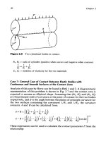
later). Therefore, the deformation depth is calculated by (Fig.
7.18):
hd
=
RsinOtanO
8
is
very small, therefore:
(7.34)
The variation of the deformation depth with load is shown in Fig.
7.19.
Then the effective modulus of elasticity of the coated surface is proposed as:
(7.35a)
where
Eh
=
modulus
of
elasticity of base material
E,.
=

modulus of elasticity of coating material
E,
=
modulus of elasticity of coated surface
h,.
=
coating film thickness
hd
=
elastic deformation depth
r
=
constant (it is found that
r
=
13
best fits the test data)
282
Chapter
7
Figure
7.18
The contact of the shaft and the coated disk.
0.006
0.005
0.004
E
0.003
U
r

A
Y
0.002
0.001
,
+Steel-Tin
-
-A-
Steel-Copper
'
-Steel-steel
4-
Steel-Chromium
0.000 a
I
.
*
fi
a
I
a
'
a
'
'
a
'
'
'
' '

'
.
I
'
a
'
*
I
a
'
.
a
I
1
.o
1.5
2.0
2.5
3.0
3.5
4.0
W
(Nlm
~10')
Figure
7.19
Variation of deformation depth on coated surface
with
load.
RollinglSliding

Contacts
EC
8
Eb
283
_______
_
# *
*-e-
0-
0
0
0
4
0
I
#
f
#
#
I
I
f
0
8
I
I
I
I
I

I
I
I
I
I
I
I
I
I
I
I
I
I
I
I
I
I
I
0
10
20
30
40
50
60
Figure 7.20 shows the variation of effective modulus of elasticity of coated
surface for different values of
h,/hd.
The effective combined modulus of
elasticity is therefore calculated by

(7.3
5
b)
For most metals used in engineering, the variation of
U
is small, and conse-
quently, the variation in
1
-
v2
is smaller. Therefore, no significant error is
expected from using the Poisson’s ratio
of
the base material
or
the coating
material.
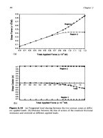
Figures 7.21 and 7.22 show the comparison of the calculated coefficient
of
friction in pure rolling conditions with the test results for chromium and
steel. Figure
7.23
shows the calculated coefficient of friction in the thermal
regime compared with test results for tin, steel, chromium, and copper.
Figure 7.24 shows the calculated coefficient of friction in the thermal regime
compared with the results from Drozdov’s
[
171,
Cameron’s
[

181, Kelley’s
[
191, and Misharin’s
[20]
experiments. Figures 7.25-7.28 show sample com-
parisons of the experimental results with the curves, which are constructed
by using the calculated
f,,f,,
andf,, and appropriate curves against slide/roll
ratios. Figure 7.29 shows the comparison of Plint’s test data with prediction.
It can
be
seen that the correlations are excellent.
284
0.08
0.06
0.04
y.
0.02
0.06
Chapter
7
0
U=0.303mlr
.
U=l.44m/s
A
U=2.76mls
-
0

U=0.303ml8
.
u=1.44mls
A
U=2.76m/s
0
n
0
U
8
8
.
A
A
I
A
0.00
1
I
I
I
I
I
0.5
1
.o
1.5
2.0
2.5
3.0

3.5 4.0
W
(N/mx106)
0.04
cc
0.02
0.00
0.5
1.0
1.5
2.0
2.5
3.0
3.5
4.0
(b)
W
(Nlm
xl
06)
Figure
7.21
with prediction for
(a)
tin;
(b)
chromium;
(c)
copper; (d) steel.
Comparison of experimental coefficient

of
rolling friction
vs.
load
Rolling} Sliding
Contacts
0.08
0.06
285
0
U=0.303m/r
U=1.44mlfs
A
U=2.76mls
-
0.08.
0.06
0.04
cc
0.02
O*O2[7
,
-
;,
I
;,
I
0.00
0.5
1

.o
1.5
2.0
2.5 3.0 3.5
4.0
(c)
W
(NImxl
0')
0
U=0.303m/s
rn
U=l.44m/s
A
U
=
2.76
m/s
-
-
A
-
286
Chapter
7
0.04
Ic
O*02!
0
W-94703Wm

W=l69408)(lm
A
W=284109N/m
v
W
=
378812
N/m
-
:
0.00
I
I
I
I
I
I
0.0
0.5 1
.o
1.5 2.0 2.5 3.0
(a)
W
(Nlmxl
0')
0.08
i
0.06
0
W

=
94703
Nlm
m
W=189406Nlm
A
W=284109Wm
v
W
=
310092
N/m
0.0
0.5
1
.o
1.5
2.0
2.5
3.0
(b)
w
(N/m
JC~
04
Figure
7.22
speed
with prediction for
(a)

tin;
(b)
chromium;
(c)
copper;
(d)
steel.
Comparison of experimental coefficient of rolling friction
vs.
rolling
RollinglSliding Contacts
'
-
287
0.04
cc
0.02
0.08
I
-
-
0.06
0.08
0.06
0.04
cc
0.00
.
0
W=94703N/m

W
=
189406N/m
A
W
=
284109
N/m
v
W
=
378812 N/m
-
-
0
W=94703N/m
m
W=l89406Nlm
A
W=284409Nlm
v
W
=
376812
Wm
0.00
I
1
I
I I

0.0 0.5
1
.o
1.5
2.0 2.5
(c)
U
(mw
288
Chapter
7
0.06
0.08
8
-
I
8
8
I
A
-
0
0
0
0
0.04
r
0.02
'
0.06

0.00
I
I
I
I
I
I
I
I
I
I
-
I
-
A
A
A
I
.

0.0
0.5
1.0
1.5
2.0
2.5 3.0 3.5 4.0
(a)
W
(N/mx106)
0.04

cc
0.02
-
-
0
U=0.303mlr
U3:1.44ml8
A
U+2.76ds
0.00
I
I I
I
I
I
I I
0.0
0.5
1.0
1.5
2.0
2.5
3.0
3.5 4.0
(b)
W
(Nlm
XI
07
Figure

7.23
Comparison
of
experimental coefficient of thermal friction
vs.
load
with prediction for
(a)
tin;
(b)
chromium; (c) copper; (d) steel.
RollinglSliding
Contacts
0.08
0.06
0.04
cc
0.02
289
L
0
U=O.303mls
U=1.44mls
A
U=2.?6mls
0
U
0
-
0

-
I
8
m
A
A
A
-
0.00
1
I
I
I I
I I
0.5
1
.o
1.5
2.0
2.5
3.0
3.5
4.0
(c)
W
(Nlmxl
06)
U
=
1.44

m/s
0.06
0.04
-
Ic
8
r
0.00
1
I
I
I
I
I
I
0.5
1.0 1.5
2.0
2.5
3.0
3.5 4.0
(d)
W
(Nlmxl
OS)
290
Chapter
7
(a)
f

(predicted)
0.08
0.07
0.06
A
0.05
c
‘t
am
9
0.04

E
0.03
I
I I I I
0.00
0.01
0.02
0.03
0.04
0.05 0.06
0.07
0.08
(b)
f
(predicted)
Figure
7.24
Comparison

of
test data with prediction: (a) Cameron;
(b)
Misharin;
(c) Kelley;
(d)
Drozdov.
Rolling/ Sliding Con
tact
s
0.08
0.07
0.06
0.05
-
8
0.04
Q)
Y
0.03
0.02
0.01
0.00
n
0.00
O.O?
0.02
0.03
0.04
0.05

0.06
0.07
0.08
(a
f
(predicted)
29
I
(d)
f
(predicted)
0.08
W
=
94703
Nhn
0.04
0.03
0.02
292
Chapter
7
0.0
0.1
0.2
0.3
0.4
A
0
8

A
V
A
Tin
Chnnnium
COpQer
Steel
0.08
W
=
94703
Nh
0.07
0.06
0.05
0.04
0.03
0.02
rc
-
U
=
0.303
mh
0
A
-
U
=
0.303

mh
Y
o
Tin
Chromium
A
copper
Tin
Chromium
Copper
0.01
v
Steel
0.00-
-
'
a
'
'
I
'
'
*
'
I
'
' '
'
I
'

'
0.0
0.1
0.2 0.3 0.4
(b)
z
Figure
7.25
0.303
mjsec): (a) experimental;
(b)
calculated.
Coefficient of friction
vs.
slide/roll ratio
(
W
=
94,703
N/m,
U
=
RollinglSliding
Con
facts
293
v
Steel
.""""l"'"""
0.0

0.1
0.2
0.3
0.4
(a)
Z
0.06
0.05
o
Tin
Chromium
A

A
0.0
0.1
0.2
0.3
0.4
(b)
z
Figure
7.26
Coefficient of friction
vs.
slide/roll ratio
(W
=
94,703
N/m,

U
=
0.303
m/sec): (a) experimental;
(b)
calculated.
294
Chapter
7
0.08
I
W=87M12Nhn
0.07
U=2.7Omh
c
ofln
=
chromium
Ir
coPP@r
9
steel
0.0
0.1
0.2
0.3
0.4
(a)
Z
-

0.06
~~
0.05
0.04
-
-
c
0.03
0.02
0.01
0.00
Ur2.7Omh U
=
2.76
mh
-
I
0
Tin
Chromium
9
steel
A
COPPM
li l l.l
0.0
0.1
0.2
0.3
0.4

(b)
Z
Figure
7.27
2.76 mlsec): (a) experimental;
(b)
calculated.
Coefficient
of
friction
vs.
slide/roll ratio
(
W
=
378,8
12
N/m,
U
=
0
Steel
*."t""t.*"""
0.0
0.1
0.2
0.3
0.4
(a)
Z

0.08
0.07
0.06
0.05
0.04
0.03
0.02
0.01
0.00
cc
W
=378812
Nhn
U=l.Umh
0
Tin
rn
Chromium
*
Copper
v
Steel
.1.l.1.,1 1 ,.
0.0
0.1
0.2
0.3
0.4
(b)
Z

Figure
7.28
Coefficient of friction
vs.
slidelroll ratio
(W
=
378,812
N/m,
U
=
1.44
m/sec):
(a)
experimental;
(b)
calculated.
296
Chapter
7
rc
0.10
I
0.09
0.08
0.07
0.06
0.05
0.04
0.03

0.02
0.01
0.00
0.00
0.05 0.10 0.15
0.20
0.25
z
Figure
7.29
Comparison
of
Plint's test data with prediction.
7.7.6
Surface
Chemical
layer
Effects
All the test data used
so
far are obtained from ground or rougher surface
contacts. The chemical layer on the contact surfaces resulting from the
manufacturing process and during operation is ignored because it wears
off
relatively quickly on a rough surface, especially at the real areas
of
contact where high shear stress is expected. On the other hand, the surface
chemical layer can be expected to play an important role in smooth surface
contacts. The properties of the contact surfaces are affected by this chemical
layer because it can remain on the surfaces more easily than on a rough

surface. In this case, Eq.
(7.27)
can be used to account for this effect.
Cheng
[7],
Hirst
[8],
and Johnson
[9]
conducted experimental investiga-
tions on very smooth surface contacts. All the contact surfaces were super-
finished. The
A
values are roughly between
80
and
100
for Cheng's test,
50
and
60
for Hirst's test, and
40
and
60
for Johnson's test.
(A
=
ho/Sc,
and

Sc
=
,/:fs:,
where
S1
and
S2
are surface roughness of contact surfaces,
CLA.)
Because the surface chemical layers usually are very thin, they are
assumed to have little effect on the elastic properties of the surfaces.
Rolling/ Sliding
Contacts 297
-6-
-5
-
4-
-3
-
-2
-
-1
-
However, they affect the temperature rise in the contact zone significantly.
In order to use
Eq.
(7.27) to account for this effect, the thermal-physical
properties and thickness of the chemical layer are needed. Because these
values are not known, the following thermal-physical properties are used
as an approximation:

tl
p
=
3792 kg/m3
E
=
3.45
x
10"
Pa
K
=
0.15
W/(m
-
"C)
c
=
840 J/(kg
-
"C)
A
Johnron*r Test
0
Cheng'r Test
Hirrt'rTert
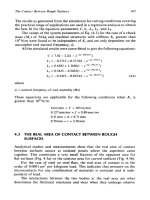
TheS, values from the above tests are used to find the thickness of the
corresponding chemical layers inversely. The result is shown in Fig. 7.30.
It is found that the thickness decreases as the load increases as expected
because the higher the load, the higher the shear stress in the lubricant,

which results in a thinner chemical layer. In Figs 7.31-7.33, the test data
are compared with prediction. It can
be
seen that the chemical layer makes a
-0
I
I
I
I
I
I
I
I
I
0
.o
2.0~10~
4.Ox1O6
6.0~1
OS
8.0x105
1
.ox1
o6
W
(N/m)
Figure
7.30
Inversely calculated surface chemical layer thickness vs. load for
superfinished surface contacts (roughness

=
1
pin.
CLA).
298
Chapter
7
0.05
0.04
0.03
0.02
-
-
-
-
0.01
Figure 7.91
Comparison
of
Cheng's experimental data with prediction.
-
i
i
0
2SOp.l
0
mpd
0
1Mp.l
A

ll5pd
i
16
-
Hhrs
Data
A
C.ku).t.df,withoutm#.r.thof.mlyrr
14
-
e
CJoul.tedf,wittlGono#.rclbknof.~by.r
x
C.lo~t.df".ndi
0
c.kul.t.df,
12
-
n
E
10-
3
-
8-
d
5
E
%
6-
I=

%
0.38
GPa
8
A
A
A
.
I
8
I
8
I
1
0.0
0.5
1
.o
1.5
2.0
Sliding Speed
(rnrs)
Figure 7.92
Comparison
of
Hirst's test data with prediction.
Rolling} Sliding Contacts
299
0.06
e

t
Q)
‘6
0.05
5
8
0.04
#
0*03
C
0.02
0.01
0.00
0.08
I
-
-
B,
Q
B,
;
:
B,
-
B,
iIi
-
-0
0
1.38GP8

A
1.01OP.
0
0.76OPa
0
0.60
V
0.43GP.
I
I
I
I
I
I
0
IK
I
0.07
I
0
10
20
30
40
50
60
70
Sliding
Speed,
(U,-U,)

(ink)
Figure
7.33
Comparison
of
Johnson’s experimental data with prediction.
great difference in the coefficient of friction for conditions with large
A
ratios
(>40)
in the thermal regime. Load can have a significant effect on the
chemical layer thickness and Fig.
7.30
can be used for evaluating the thick-
ness as a function of normal load.
7.7.7
General Observations
on
the
Results
The empirical formulas were checked for different regimes of lubrication,
surface roughness, load, speed, and surface coating. The formulas were used
for evaluating rolling friction, and traction forces in the isothermal, non-
linear, and thermal regimes of elastohydrodynamic lubrication. Because of
the current interest in surface coating, the formulas were also applied for
determining the coefficient
of
friction for cylinders with surface layers of any
arbitrary thickness and physical and thermal properties.
It can be seen from the empirical formulas that:

1.
It appears that in general, the slide/roll ratio has little direct effect
on the coefficient of friction in the thermal region (slidelroll
>
0.27).
300
Chapter
7
2.
The surface roughness effect
is
treated in this study as a function
of the surface generating process rather than the traditional
surface roughness measurements.
The oil film thickness is found to be better represented for friction
calculation in a nondimensional form by normalizing it to the
effective radius rather than the commonly used film thickness to
roughness ratio
A.
Coating has a significant effect on the temperature rise in the
contact zone. This is represented by a factor
B,
as shown in
Eq.
(7.3
0).
Coating has an effect on the modulus of elasticity as shown in
Eq.
(7.35).
This

is
represented by using an effective modulus of elas-
ticity for the coated surface. For tin (whose modulus of elasticity
differs from that of the base material most significantly among
the three coating materials used), this correction produces
a
50%
increase in the effective modulus of elasticity.
3.
4.
5.
7.8
PROCEDURES
FOR
CALCULATION
OF
THE COEFFICIENT
OF
FRICTION
7.8.1
Unlayered Steel-Steel Contact Surfaces
1.
Given: contact surface radii
rl,
1-2
(m, in.)
Surface velocities,
U1,
U,
(mlsec, in./sec)

Dynamic viscosity
of
lubricant oil at entry condition
qo
(Pa-sec,
reyn)
Load
F
(n, lbf)
Surface roughness
S1,
S2
(m
CLA, in. CLA) or manufacturing
processes
Density of lubricant
p
(kg/m3, (lb/in.3)
x
0.0026)
Modulus of steel
E
(Pa, psi)
Contact width of surfaces
y
(m, in.)
Poisson’s ratio for steel
v
(dimensionless)
Pressure-viscosity coefficient of lubricant

a!
(
1
/Pa,
1
/psi)
2.
Calculate:
E
Effective modulus
of
elasticity
E’
=
-
1-3
U1
+
U2
2
Mean rolling velocity
U
=
~
Rolling/Sliding
Con
lac
ts
30
I

3.
4.
5.
6.
7.
8.
9.
rl r2
Effective radius
R
=
-
YI
+r2
F
Load per unit width
W
=
-
Y
Find
Sr.2,
from Fig. 7.13a by using
S1
and
S2
(or by manu-
facturing processes). For
S
<

0.05
pm, take
S,,
=
0.05
pm. Then
Calculate dimensionless
U,
q,
W,
S
from Eqs. (7.17bt7.20).
Calculate coefficient of rolling friction
.fi
from
Eq.
(7.21).
Calculate coefficient of friction in the nonlinear region and its
location.f, is calculated from Eq. (7.22),
z*
is calculated from
Eq.
(7.23).
Calculate minimum oil film thickness
ho
from
Eq.
(7.26), where
G
=

@E'.
Find.fo from Fig.
7.12.
Find
(S,,(./R)(,
from Fig. 7.13b. Calculate
coefficient
of
thermal friction
fr
from Eq. (7.24).
Use.fr,.fn,
z*,
and
.fi
to construct the coefficient of friction curve
versus sliding/rolling ratio,
as
in Fig. 7.1 1, where sliding speed
=
I
U]
-
U,
I,
and rolling speed
=
U.
s,,
=

4-
7.8.2
Layered Surfaces
1.
Given: contact surface radii
rl,
rl
(m, in.)
surface velocities
U1
,
U2
(m/sec, in./sec)
load
F
(N,
lbf)
surface roughness
S,,
S2
(m
CLA,
in.
CLA)
or manufacturing
processes
density of lubricant
p
(kg/m3, (lb/in.3)
x

0.0026)
modulus of steel
E
(Pa, psi)
contact width
of
surface
y
(m, in.)
Poisson's ratio for steel
U
(dimensionless)
Lubricant oil properties:
Thermal conductivity
KO
(W/m-'C), (BTU/(sec-in OF))
x
9338)
Specific heat
CO
(J/(kg-"C), (BTU/lb-OF)
x
3,604,437)
Pressure-viscosity coefficient
a
(I/Pa,
l/psi)
Temperature-viscosity coefficient
/3
(1

/"C,
1
/OF)
Dynamic viscosity at entry condition
qo
(Pa-sec, reyn)
Disk
1
base material properties:
Modulus of elasticity
Ehl
(Pa, psi)
Poisson's ratio
uhl
(dimensionless)
302
Chapter
7
Thermal conductivity
Kbl
(W/(m-OC), (BTU/(sec-in-OF)
x
9338)
Specific heat
cbl
(J/(kg-"C), (BTU/(lb-OF)
x
3,604,437)
Density
pbl

(kg/m3, (lb/in.3)
x
0.0026)
Disk
1
surface material properties:
Modulus of elasticity
ECl
(Pa, psi)
Poisson's ratio
ucl
(dimensionless)
Thermal conductivity
Kcl
(W/(m-"C), (BTU/(sec-in OF)
x
9338)
Specific heat
ccl
(J/(kg-"C), (BTU/(lb-OF)
x
3,604,437)
Density
pcl
(kg/m3, (lb/in.3)
x
0.0026)
Thickness
hCl
(m, in.)

Disk
2
base material properties:
Modulus of elasticity
Eb2
(Pa, psi)
Poisson's ratio
ub2
(dimensionless)
Thermal conductivity
Kb2
(W/(m-OC), (BTU/-sec-in "F)
x
9338)
Specific heat
cb2
(J/kg-"C), (BTU/(lb-OF)
x
3,604,437)
Density
pb2
(kg/m3, (Ib/in.3)
x
0.0026)
Disk
2
surface material properties:
Modulus
of
elasticity

Ec2
(Pa, psi)
Poisson's ratio
uc.
(dimensionless)
Thermal conductivity
Kc2
(W/(m-OC), (BTU/(sec-in,-"F)
x
9338)
Specific heat
cc2
(J/(kg-"C), (BTU/(lb-OF)
x
3,604,437)
Density
pc2
(kg/m3, (lb/in.3)
x
0.0026)
Thickness
hc2
(m, in.)
Steel properties:
Modulus
of
elasticity
Es
(Pa, psi)
Poisson's ratio

vs
(dimensionless)
Thermal conductivity
Ks
(W/(m-OC), (BTU/(sec-in OF)
x
9338)
Specific heat
cs
(J/(kg-"C), (BTU/(lb-OF)
x
3,604,437)
Density
ps
(kg/m3, (lb/in.3)
x
0.0026)
Bulk temperature
Tb
(K,
R)
(K
=
"C
+
273.16)
Use previous section
to
calculate
fr

for steel-steel contact
sur-
faces. Substitute
ATs,
Ks,
cs,
ps,
and
Es
for
AT,
K1,
c1,
p1,
El
and
K2,
c2,
p2,
E2
in
Eqs.
(7.27)
and
(7.28),
where
f
is replaced
byf,,
L

is replaced by
L
=
32J'm.
2.
U1
+
U2
3.
Mean rolling velocity
U
=
-
2
rl
r2
Effective radius
R
=
-
rl
+
r2
Rolling/Sliding
Contacts
303
F
Load per unit width
W
=-

X
Effective modulus of elasticity
-
-
-
WR
4. Half contact width
6
=
1.6,/-
E'
5.
Calculate
hd
by using Eq. (7.34).
6. Substitute
Ebl
,
Ecl
,
hcl
for
Eb,
E,,
h,
in Eq. (7.35) to calculate
Eel.
Substitute
Eb2, Ec2,
hc2

for
Eb,
Ec,
h,
in Eq. (7.35) to calculate
Ee2.
7. Calculate the effective modulus of elasticity of the layered
surfaces by:
8.
9.
10.
11.
12.
13.
14.
15.
16.
17.
18.
Find
Sel,
Se2
from Fig. 7.13a by using
Sl
and
S2
(or
by manu-
facturing processes).
For

S
<
0.05
pm take
Se
=
0.05
pm.
Then
S
-
ec
=
,/Sx.
Calculate dimensionless
U,
q,
W,
S
from Eqs. (7.17)-(7.20)
except that
E'
is replaced by
E,&.
Calculate coefficient
of
rolling friction
fr
from Eq. (7.2 1).
Calculate coefficient

of
friction in the nonlinear region and its
location
fn
is calculated from
Eq.
(7.22),
z*
is calculated from
Eq. (7.23).
Calculate minimum oil film thickness
ho
from Eq. (7.26), where
G
=
aE,I,.
Calculate
E
by using Eq. (7.28), where
z
=
0.27.
Calculate
A
T,
by Eq. (7.27), where
Kl
,
c1,
p1

,
El
are replaced by
L
=
26,f
=f!
from step 2 for steel-steel contact surfaces.
Calculate
D1
by using Eq. (7.29) where K,
c,
p,
U
are substituted
by
K1,
c1
,
pl,
El.
Use Eq. (7.30) to calculate
p1
where
h,
=
hCl
,
Calculate
D2

by using Eq. (7.29) where
K,
c,
p,
U
are substituted
by
K2,
c2,
p2,
E2.
Use Eq. (7.30)
to
calculate
p2
where
h,
=
hr2,
Calculate
AT,
by using Eq. (7.31) where
/?
=
(PI
+
P2)/2.
Use Eq. (7.32) to calculate
a
and

6
for theparticular lubricant
as follows. Suppose that the viscosity
is
rnl
at T1 and m2 at
T2 (where T1 and
T2
are absolute temperature, say,
K
=
273.16
+
"C, ml and m2 are kinematic viscosity in centi-
&I*
cc19
Pcl9
&I*
K2
9
c2
*
P2
*
E2
are replaced by
Kc2
*
cc2
*

Pc2
,
Ec2
*
D
=
01.
D
=
02.
304
Chapter
7
19.
20.
21.
22.
23.
stokes), substitute ml, Tl and
m2,
T2 into Eq. (7.32), respec-
tively, and solve these two linear equations simultaneously to get
a
and
6.
(If
lubricant is
SAE
10,
SAE

20,
SAE
30,
SAE
40,
SAE
50,
SAE
60,
or
SAE
70, use Table 7.3.)
Use Eq. (7.32) to calculate the viscosity
q
at temperatufe
T,(q
=
pou
where
po
is the lubricant density,
U
is the kinematic
viscosity).
Use Eq. (7.26) to find
ho
where
qo
=
q,

G
=
al&.
Findfo from Fig. 7.12. Find
(Sc,r/R)',
from Fig. 7.13b. Calculate
coefficient of thermal frictionf, from Eq. (7.24).
If the difference betweenf, value in step 21 andf, value in step 14
does not satisfy your accuracy requirement, go back to step 14,
replace
.ft
by
fr
value in step 21 and iterate until the accuracy
requirement is satisfied.
Use
f;.fn,
z*,
and
J
to construct the coefficient of friction curve
versus sliding/rolling ratio as in Fig. 7.1 1, where sliding speed
=
lU,
-
U21,
and rolling speed
=
U.
7.9

SOME NUMERICAL RESULTS
The following are some illustrative examples for the application of the
developed empirical formulas in sample cases.
Figure 7.34 shows calculated coefficient of friction versus sliding/rolling
ratio for different rolling speeds,
T
=
26°C (78.8"F), steel-steel contact,
ground surfaces,
S
=
0.03 pm (1 2 pin.),
W
=
378,8 12
N/m
(2
160 lbf/in.),
10W30 oil,
R
=
0.0234m (0.92 in.).
Figure 7.35 shows calculated coefficient of friction versus sliding/rolling
ratio for different normal loads, T
=
26°C (78.8"F), steel-steel contact,
ground surfaces,
S
=
0.03 pm (12 pin.), U1

=
3.2 m/sec (126 in./sec),
10W30 oil,
R
=
0.0234 m (0.92 in.).
Figure 7.36 shows calculated coefficient of friction versus slidinglrolling
ratio for different effective radii,
T
=
26°C (78.8"F), steel-steel contact
ground surfaces,
S
=
0.03 pm (12 pin.),
W
=
378,8 12 N/m
(2
160 lbf/in.),
10W30 oil, U1
=
3.2m/sec (126in./sec).
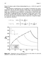
Figure 7.37 shows calculated coefficient of friction versus sliding/
rolling ratio for different viscosity, steel-steel contact, ground surfaces,
S
=
0.03 pm (12pin.),
W
=

378,812N/m (21601bf/in.), 10W30
oil,
U1
=
3.2 m/sec (126 in./sec),
R
=
0.0234 m (0.92 in.).
Figure 7.38 shows calculated coefficient of friction versus sliding/
rolling ratio for different materials,
T
=
26°C (78.8"F), ground surfaces,