Friction and Lubrication in Mechanical Design Episode 2 Part 6 doc

Case Illustrations
of
Surface Damage
355
force effects of solid rollers cause an additional loading at the outer race
contact (and a second-order, not significant unloading at the inner race
con tact).
Harris and Aaronson
[40]
made analytical studies of bearings with
annual rollers to investigate the load distribution, fatigue life, and the skid-
ding of rollers. Their work shows that hollow rollers increase the fatigue life
of the bearing and decrease the skidding between the cage and roller set.
They suggested that attention should be paid, however, to the bending stress
of the rollers and to the bearing clearance.
This section describes an experimental study undertaken by Suzuki and
Seireg
[41]
to compare the performance of bearings with uncrowned solid and
annular rollers under identical laboratory conditions. Bearing temperature
rise and roller wear are investigated in order to demonstrate the advantages
of using annual rollers in applications where skidding can be a problem.
Test
Bearings
The two bearings used in the study have the same dimensions and configura-
tions with the exception that one bearing has annular rollers and the other
bearing has solid rollers. The details of the bearings are given in Table
9.1.
Brass is selected as the roller material in order to rapidly demonstrate
the effect of annular rollers
on

temperature rise, and roller wear.
The ratio of the inside to the outside diameter of the hollow roller
is
taken as
0.3.
Three sets of inner rings with different outside diameters are
used for each bearing in order to produce the different clearances.
Special efforts were undertaken in machining the rollers and rings to
approach the dimensional accuracy and surface finish of conventional har-
dened bearing steels.
Test Fixture
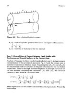
The experimental arrangement is diagrammatically represented in Fig.9.12.
the two test bearings (a) and (b) (one with hollow rollers and another with
solid rollers) were placed symmetrically near the middle plane of a shaft (c).
The shaft is supported by two self-lubricated ball bearings (d) on both sides.
A
variable speed drive is used to rotate the shaft through a V-belt (e) and
and a pulley
(f)
at one end of the shaft.
The load is applied radially
on
the outer rings (g) inside which the
bearing is placed by changing the weight
(j)
suspended at one end of a
bar (k). The latter loads a fulcrumed beam-type load divider, which is
especially designed to provide identical loads on both bearings.
A
strain

gage ring-type load transducer (i) monitors the load applied on the test
bearings to confirm the equality of the load on them at all times. Separate
356
Chapter
9
Table
Q.1
Test Bearing Specifications
Bearing outside diameter
Bearing inside diameter
Bearing width
Outer race inside diameter
Inner race outside diameter
Roller diameter
Roller length
Number of rollers
Roller inside diameter
Diameter ratio
Bearing radial clearance
Roller material
Outer and inner race material
Surface finish for rollers and races
4.3305
in.
1.9682
in.
1.06
in.
3.719
in.

2.5658
in.
2.5637
in.
2.5620
in.
0.5766
in.
0.659
in.
12
0.1719
in.
0.3
0.0021
in.
0.0038
in.
Brass
Mild steel
8-10
pin rms
(10.99947
cm)
(4.999228
cm)
(2.6924
cm)
(9.4462
cm)

(6.517132
cm)
(6.51 1798
cm)
(6.50478
cm)
(1.464564
cm)
(1.67386
cm)
(0.436626
cm)
(0.005334
cm)
(0.009653
cm)
Load
Figure
9.1
2
Diagrammatic representation of experimental setup for dynamic test.
Case Illustrations
of
Surface Damage
35
7
oil pans (1) are placed below each of the test bearings. Oil is filled to the level
of the centerline of the lowest roller. Copper+onstantan thermocouples are
used to measure the bearing temperatures as well as the oil sump tempera-
ture. The bearing thermocouples are embedded 30" apart at 0.01 in.

(0.25mm) below the surface of the outer rings where rolling takes place.
The thermocouples are connected to a recorder
(s)
through a rotary selec-
tion switch (q), and a cold box (r).
Results
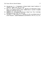
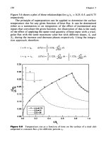
Figure 9.13a shows the time history of the outer race temperature rise for
the bearing with annular rollers. Steady-state temperature conditions are
reached after approximately two hours. Figure 9.13b shows the bearing
temperature rise as well as oil temperature rise at steady state conditions
for a shaft speed of 1000 rpm. The temperature rise for both solid rollers and
annular rollers are essentially the same at this speed. At speeds of 2000 rpm
and 3000 rpm, on the other hand, the temperature with solid rollers is higher
than that with annular rollers. The temperature rise differences are most
pronounced at 2000 rpm.
Wear Measurement
The radioactive tracing technique used in the test is similar to that used by
L.
Polyakovsky at the Bauman Institute, Moscow
for
wear measurement
in
the piston rings of internal combustion engines.
The test specimens (hollow or solid rollers) are bombarded by a high-
energy electron beam emitting gamma rays. The strength of the bombard-
ment is governed by the energy of the electron beam, the exposure time, and
the material of the specimen. The radioactivity, which naturally decays with
time, is also reduced with wear of the bombarded surface. The rate of
reduction of the radioactivity is approximately proportional to the depth
of wear. The amount of wear can therefore be detected by monitoring the

radioactivity of the specimen and using a calibration chart prepared in
advance of the test. The main advantage of this method is the ability to
detect roller wear without disassembling the bearing. The disassembling
process is not only time consuming, but it may also alter the wear pattern
of the test specimens.
In this study, one roller in each bearing is bombarded and assembled
with the rest of the rollers.
A
scintillation detector
(w)
is placed on the outer
surface of the outer ring of the bearing (Fig. 9.12) and a counter is used to
monitor the change in radioactivity of the bombarded rollers. The diameter
of rollers is periodically measured using an electric height gage to check the
accuracy of the radioactive tracing technique.
358

60-
E:
50-
e
w-
40-
2.
3
30-
a
20-
10-
0

$-
L
Chapter
9

Bearing
Oil
I
I
I
1
I
I
70
-
.
SAE50Oil
I
I
3000
60-
Bearing Temperature
-
rpm
50-
e
a
40-
3
30-

8-
I'
Y
Y
-
K
loo0
!i
20:
- -
0-
-

Q

Q
2000
______
x

x "x
1000
E-
10-
0
1
I
I
I
1

.o
1.5
2.0
2.5
0.0
0.5
Time (hrs)
Figure
9.13
(a) Temperature rise-time history for the bearing with annular roll-
ers. (b) Temperature rise at steady-state conditions.
The shaft speed for the wear test is selected as
3000
rpm
and kept
unchanged.
SAE
IOW
oil is used as the lubricant for the test bearings
to
accelerate the roller wear. The bearing outer race temperature and
oil
tem-
perature are monitored throughout the test.
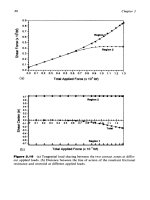
Figure 9.14a shows a comparison
of
the wear
of
the roIIers during the
test.

As
can be seen from the figure, the wear of the annular
rollers
is
Case Illustrations of Surface Damage
40
-
359
-

-
Sdid
Roller
Bearing
-A-
Annular
Roiler Bearing
o.oO06
1
1
Flgure
9.14
oil.
(a) Roller wear.
(b)
Temperature difference between bearings and
considerably lower than that of the solid rollers. It should be noted that
after an initial running period
of
30

hours, the oil was changed and a con-
siderably lower rate of wear resulted. The wear rate during this phase of the
test is shown as
5.7
x
10-7
in./h
(14.5
x
10-6
mm/h) for the hollow roller as
compared to
8
x
10-7
in./h
(20.4 x
10-6
mm/h) for the solid roller.
It was observed throughout the test that the wear detected using radio-
active tracing technique is slightly higher than that measured directly using
the electric height gage. The reason may lie in the fact that the wear detected
by the radioactive tracing technique
is
an average wear, which includes the
360
Chapter
9
indentations due to local pittings or flakings. Consequently,
if

the interest is
to study the effect of wear on the change of bearing clearance, it would be
more appropriate to use the height gage for measuring the dimensional
change. On the other hand,
if
the interest is to investigate the surface
damage, the radioactive tracing technique would be a good tool for this
purpose. Better accuracy can be expected with this technique when steel
rollers are used. Gamma-ray emission is stronger with steel and conse-
quently the influence
of
the radioactivity existing in the natural sp: :e on
the results is reduced.
The temperature rise in the bearings and oil during the wear est is
shown in Fig. 9.14b. The temperature of the outer race
of
the solid roller
bearing is shown to be consistently higher than that of the annular roller
bearing at all times.
It is interesting to note that the annular roller exhibited a small number
of
local pits scattered on the rolling surface. In the solid roller, however, a
large number
of
pits were observed in the rolling direction only at the central
region
of
the rolling surface. This may also be due to the cooling effect at the
ends
of

the rollers.
9.3
SURFACE TEMPERATURE, THERMAL STRESS, AND WEAR
IN
BRAKES
The high thermal loads, which are generally induced in friction brakes, can
produce surface damage and catastrophic rotor failure due to excessive sur-
face temperatures and thermal fatigue. The temperature gradients and the
corresponding stresses are functions of many parameters such as rotor geo-
metry, rotor material, and loading history.
Due
to
the wide use of frictional brakes, an extensive amount of work
has been undertaken to improve the performance and extend the life of their
rotors. Some research has been aimed towards studying the effects of rotor
geometry on the temperature and stress distribution using classical analyti-
cal [42-45] or numerical [46-521 methods. Other studies have concentrated
on investigating the effects of rotor materials on the performance of the
brake
[53-551.
The efforts to improve the automobile braking system performance and
meet the ever increasing speed and power requirements had resulted in the
introduction
of
the disk braking system which is considered to be better than
the commonly used drum system.
A
newer system which
is
claimed to be

superior to both of its predecessors is now being introduced. The crown
system [56] which can be viewed as a cross brake, with a drum rotor and a
Case Il[ustrations
of
Surface Damage
361
disk caliper, combines the advantages of both drum and disk systems. It has
the loading symmetry of the disk caliper which results in less mechanical
deformation.
It
also has the larger friction surface areas and heat exchange
areas
of
the drum which result in better thermal performance and lower
temperatures.
A
study by Monza
[56],
in which the disk and crown are com-
pared, indicated that more weight and cost reduction are attainable by using
the crown system. Moreoever, under similar testing conditions, the crown
rotor showed
10-20%
lower operating tempratures than its counterpart.
This section is aimed at investigating the thermal and thermoelastice
performance
of
rotors subjected to different types of thermal loading.
Although there are many procedures in the literature for the analysis
of

temperature and stress in brake rotors based on the finite element method
[l,
3,
8,
91,
these procedures would require considerable computing effort.
Efficient design algorithms can be developed by placing primary emphasis
on the interaction between the design parameters with sufficient or reason-
able accuracy. Sophisticated analysis can then be implemented to check
the obtained solution and insure that the analytical simplifications are
acceptable.
For
the thermoelastic analysis
in
this section, a simplified one-dimen-
sional procedure is used. The rotor
is
modeled as a series of concentric
circular rings of variable axial thickness. Furthermore, it is assumed that
the rotor
is
made of a homogeneous isotropic material and that the axial
temperature and stress variations are negligible. The procedure first treats
the thermal problem to predict the temperature distribution which is then
used to compute the stress distributions.
9.3.1
This algorithm used to calculate the temperature rise is a simplified one-
dimensional finite difference analysis. The analysis consideres the transient
radial temperature variations and neglects both axial and circumferential
variations. The rotor, which is subjected to a uniform heat rate,

Qr
at its
external, internal or both cylindrical surfaces dissipates heat through its
exposed surfaces by convention only. The film coefficient depends only on
the geometrical parameters.
The proposed analysis
is
based on the conservation of energy principles
for a control volume. This can be stated as:
Temperature Rise Due to Frictional Heating
where
Qin
and
Qour
are the rate of energy entering and leaving the volume,
by heat conduction and convection respectively and
Qslorcd
is the rate
of
362
Chapter
9
energy stored in the volume. For the shaded element
of
Fig. 9.15, Eq. (9.4)
with appropriate substitution becomes:
where
Qc,n
and
&+,

are heat quantities entering and leaving the volume by
conduction, and
Qv,n
and
Qd,n
are geometry dependent convection heat
quantities entering and leaving the body depending on the surrounding
temperature,
T,.
With a current temperature rise above room temperature,
T,,,
at the
interface
M,
one can solve for the future temperature rise, at time
t
+
1,
for
the same location
[57]:
where
k
PC
B
=
-
is the thermal diffusivity
v,n
T

‘n
C.L.
7
rIl-1
I
1
Figure
9.1
5
Diagram used
for
the temperature algorithm.
Case Illustrations
of
Surface Damage
363
Similar expressions can be obtained for the temperature at the inner and
outer surfaces. The temperature rise in the next time step at the outer
radius is:
(9.7)
and the temperature rise in the next time step at the inner surface is
obtained by replacing all the
2,O
and
U
subscripts in Eq.
(9.7)
by
m,
i,

and
I,
respectively.
In the above equations
Ao,
A,,
and
A,
are the cylindrical areas of the
outer, inner, and interface surfaces, respectively.
Au,,
and are the ring
side areas, upper, and lower halves.
Ad,,
is the area generated by the thick-
ness difference between two adjacent rings (refer to Fig.
9.15). As
can be
seen, the above algorithm can easily be modified to allow for any variations
in heat input, convective film, and surrounding temperatures with location
and time.
9.3.2
The Stress Analysis Algorithm
The geometrical model of this algorithm is identical to that of the tempera-
ture algorithm. For this analysis, both equilibrium and compatibility con-
ditions are satisfied at the rings interfaces. Considering the inner and outer
sides of the interface
rn+l
of Fig.
9.16,

the continuity condition (or strain
equality) can be expressed
as
a
function of the corresponding stresses as
follows
[58,
591:
where
0
(of,n+l)
,
(of,n+,)’
=
tangential stresses at the outer and inner side of interface
r,+I,
respectively
0
,
(o~,~+~)’
=
thermal stresses at the corresponding locations
364
Chapter
9
!I
c
1-
-
In*'

I
Tl
I
m
i
rL.L.
Figure
9.16
stress algorithm.
Representation
of
the disk geometry and the notations used in the
The radial stress
sures
on
both sides
of
the interface, can be derived as:
at the radius
I-,,+~,
which is the average of the pres-
The tangential component
o,,~+~
is calculated by averaging the stress
on
both sides of the interface as:
(9.1
I)
Case Illustrations
of

Surface Damage
365
where
where
0,
is a geometry function given by
0,
=
(r,,/r,,+,)*.
Equations
(9.9)
and
(9.10)
are used to determine the radial and tangential stress distribu-
tions. Substitution in
Eq.
(9.1
1)
for each node produces a set of simulta-
neous equations to be solved for the known boundary pressures
P2
and
P,,
to give the radial distribution in the disk. This set of simultaneous equations
is solved by assuming two arbitrary values for
P3
and using linear interpola-
tion or extrapolation to satisfy the pressure
P,,,
at the inner boundary [52].

The temperature and stress algorithms are then coupled such that the
temperature distribution
is
automatically used in the stress algorithm. This
approach makes it possible to incorporate material properties and heat
convectivity that are geometry and temperature dependent
[SS,
591.
Similar algorithms for disk brakes are given in Refs 60-62.
9.3.3
Numerical Examples
The coupled temperature-stress algorithm is used, as a module, to predict
the temperature and thermal stresses generated by a given conductive heat
flux applied at a given surface or surfaces of a disk of any given material and
geometry. Several examples are considered to illustrate the capabilities of
the developed algorithm.
The following geometrical, loading and material parameters are used in
the considered cases:
Geometry:
Disk outer radius,
ro
=
12.0in.
Disk inner radius,
ri
=
6.0in.
Disk thickness,
fmax
=

12.0
in.
366
Chapter
9
Material:
Density,
p
=
0.286
lb/in.3
Young's modulus,
E
=
30
x
106 psi
Coefficient of thermal expansion,
a
=
7.3
x
10-6
in./(in.OF)
Thermal conductivity,
k
=
26.0
BTU/(hr-ft-OF)
Specific heat,

c
=
0.1
1
BTU/(lb-OF)
Loading conditions:
Total conductive heat flow rate,
QT
(constant)
=
500,000
BTU/hr
Heating time,
t
=
180sec
Average convective heat transfer coefficient at exposed surfaces,
The case of a disk with uniform thickness is considered to investigate the
effect of the loading location on the thermal and thermoelastic behavior
of
the disk by applying the total heating load at the disk outer surface and the
inner surfaces respectively. The case where the load is shared equally
between the two surfaces is also considered, as well as the case where the
thermal load sharing between the surfaces is optimized
[59].
The tempera-
tures and tangential stresses for the three loading cases are shown in Tables
The results obtained from the report study illustrate the significant
effects of the loading location and load sharing ratio on the thermal
and thermoelastic performance of brakes. Tables

9.2-9.4
show that when
the thermal load is shared between the internal and external cylindrical
surfaces, a considerable reduction can be expected in the temperature and
stress magnitudes. It also indicates that the maximum tensile tangential
stress
is
shifted from the inner or outer surface towards the middle where
the probability of failure is reduced. The results also show that, for the
given case, internal loading produces the highest temperature and stress
h
=
5.0
BTU/(hr-ft2-"F)
9.2-9.4.
Table
9.2
The Maximum Temperatures
(OF)
for the Investigated Cases
Load condition
(:)
=
0.25
(2)
=
0.50
(:)
=
0.75

1.
Uniform thickness and external loading 448.9 465.2
0.75
2. Uniform thickness and internal loading 1345.8 787.9 469.8
3.
Uniform thickness and equal load
sharing 724.3 395.2 543.8
4. Uniform thickness and optimal load
sharing 338.9 295.9 302.8
Case Illustrations
of
Suflace Damage
36
7
Table
9.3
The Maximum Tensile Tangential Stresses (psi) for the Investigated
Cases
Load condition
(2)
=
0.25
(2)
=
0.50
(2)
=
0.75
I.
Uniform thickness and external loading

73,456.4 70,378.9 50,506.1
2.
Uniform thickness and internal loading
272,283.7 137,739.3 67,039.4
3.
Uniform thickness and equal load
sharing
13
1,164.9 54,846.
I
19,616.8
4.
Uniform thickness and optimal load
sharing
50,283.1 33,954.6 16,393.5
magnitudes. This is due to the fact that the inner surface has a smaller
area and consequently for a given heating input the flux is higher. The case
of equally shared loading between the inner and outer surfaces allows for a
larger area for the heat input, shorter penetration time, lower temperature
gradients, and consequently lower thermal stresses. Optimization
of
the
load sharing further improves the design.
9.3.4
Wear Equations for Brakes
Wear resistance in brakes is known to increase with increasing thermal con-
ductivity
of
the material, its density, specific heat, and Poisson’s ratio to its
ultimate strength and resistance to thermal shock. It

is
also known to increase
with decreasing thermal expansion and elastic modulus of the material.
The following equations can
be
used for material selection to provide
longer wear life.
Table
9.4
The Maximum Compressive Tangential Stresses (psi) for the
Investigated Cases
Load condition
(2)
=
0.25
(:)
=
0.50
(2)
=
0.75
1.
Uniform thickness and external loading
73,456.4 70,378.9 50,506.1
2.
Uniform thickness and internal loading
272,283.7 137,739.3 67,039.4
3.
Uniform thickness and equal load
sharing

13
1,164.9
54,846.1 19,6 16.8
4.
Uniform thickness and optimal load
sharing
50,283.1 33,954.6 16,393.5
368
Chapter
9
Brakes without surface coating:
a,(
1
-
p)(cpk3)”4
Wear resistance
cx
&E
Brakes with thin coated surface layer:
au(1
-
P)fi
Wear resistance
a
&E
Resistance to thermal shock:
ko0
Resistance to surface crack formation
cx
-

&E
where
(9.12a)
(9.12b)
(9.13)
E
=
modulus
of
elasticity
p
=
Poisson’s
ratio
E
=
coefficient of thermal expansion
k
=
thermal conductivity
c‘
=
thermal capacity (specific heat)
p
=
density
0,
=
ultimate strength
a.

=
resistance to crack formation (ductility)
9.4
WATER JET CUTTING AS AN APPLICATION
OF
EROSION
WEAR
One
of
the beneficial applications
of
erosion wear is the use
of
high speed
water jets for cutting and polishing. This section presents
a
review of the
literature on the subject and provides dimensionless equations for modeling
the erosion process resulting from the momentum change of
a
high-velocity
fluid. The following nomenclature is used in all the equations given in this
section.
9.4.1
Nomenclature
c
=
instrinsic speed for rock cutting
=
-

V,,JlP
rgo
kt0
Case Illustrations
of
Surface Damage
369
cf,
f
=
friction coefficient of rock
d
=
kerf width
=
2.5d0
d,
4
=
nozzle diameter
E
=
Young’s modulus of rock
g
=
9.81 m/s2, gravitational constant
go
=
grain diameter
h,

z
=
depth of cut
Ah
=
increment depth
of
cut by adding abrasive
h,v
=
depth
of
cut by plain water jet
KO
=
2100MPa,
the bulk modulus
of
the water
K1,
a
=
experiment constants
I
=
average grain size
of
the rock
n
=

porosity of the rock
(%)
p
=
jet pressure
po
=jet stagnation pressure
pc,pth
=
rock threshold pressure
Q,
=
abrasive mass flow rate
Q,,,
=
water mass flow rate based on the measurement
R
=
drilling rate
r
=
radius of rotating jet
s
=
jet standoff distance
T
=
-,
the time of exposure
U

=
feed rate
vl,
vj
=
jet velocity at nozzle exit
U,
=jet traverse velocity
/?
=
jet inclination angle
PO
=
experimentally determined constant
=
0.025
q
=
damping coefficient
q,,,
=
viscosity of the water
k
=
permeability
of
the rock
p
=
dynamic viscosity of the water

pr
=
coefficient of internal friction of rock
pH’
=
coefficient of friction for water
v
=
1.004
x
10-6
m2/s, kinematic viscosity of the water at
20°C
p
=
density of rock
po
=
liquid density
pa
=
density
of
the abrasives
(p,
=
3620
kg/m3 for garnet,
p,$,
=

998 kg/m3, density of water
0,
=
compressive strength of material
oy
=
yield strength of target material
d0
V
p,
=
2540
kg/m3 for silica sand)
3
70
Chapter
9
to
=
force required to shear
off
one grain per typical grain area
w
=
jet rotating speed
The problem of evaluating the performance of water jet cutting systems has
received considerable attention in recent years and some of the many excel-
lent studies are reported in Refs
63-70.
Several investigators developed

water jet cutting analytical models and several of these studies generated
empirical equations based on specific test results. Some of these are briefly
reviewed in the following.
Crow
[63, 641
investigated the case
of
a rock feeding at a rate
v
under a
continuous water jet with diameter
do
and pressure
po
cutting a kerf of depth
h.
The jet will fracture the rock because the pressure difference on the
exposed grains produce shear stress equal to the shear strength of the
rock. During the process, friction along the sides of the kerf causes the jet
velocity to decrease and thus the erosive power of the jet
Crow developed the following predictive equation or
The model was tested by conducting experiments on four
decreases.
the kerf depth
h:
(9.14)
different types of
rock. The results show that the proposed model gives a reasonable fit for
only one rock type, Wilkeson sandstone, over the range 0.1
<

v/c
<
50.
Based on a control volume analysis to determine the hydrodynamic
forces acting on the solid boundaries in the slot and the Bingham-plastic
model, which describes the time-dependent force displacement characteris-
tics of the solid material to be cut, Hashish and duPlessis
[65, 661
developed
a continuous water jet cutting equation
as
follows:
The maximum depth of cut
zo
achieved can be expressed as:
(9.15)
(9.16)
Case
Illustrations
of
Surface Damage
371
Equation
(9.16)
is used to determine the coefficient of friction,
c-,
experi-
mentally. Because the damping coefficient
q
in Eq.

(9.15)
is an unknown
material property, the authors had to determine
q
for a particular material
using an experimentally measured cutting depth
z
with known values of
a,,
cf,
4,
vl,
and
U.
The authors also pointed out that greater accuracy for a
particular material can be achieved by choosing the optimum rheological
model for the material.
Hood et al.
[67]
proposed a physical model of water jet rock cutting
based on experimental observations. In this model when the main force of
the jet acts on a ledge of rock within the kerf, the ledge is fractured and a
new ledge forms against which the jet acts. This process continues until the
friction along the wall of the kerf dissipates the jet energy to a value which is
insufficient to break
off
the next ledge, or until the jet moves on to the next
portion
of
the rock surface.

Considering the fact that a large number of variables influence the
erosion process, they used the factorial method
of
experimental design to
determine the jet pressure
(p)
needed to cut a kerf to a specified depth
(h)
in a
given rock type with specified nozzle diameters
(d)
and traverse velocities
(U).
The factorial method yields an empirical model for a certain material
that identifies and quantifies the relative importance of the variables. The
equations are in the form:
where
C,
K,,
K2,
and
K3
are experimental constants.
Labus
[68]
developed an empirical water jet cutting equation based on
data available in the literature. The general
form
of
his proposed equation

is:
(9.18)
While performing tests in which a plane rock surface was exposed to a
vertical stationary jet, Rehbinder
[69,
701
observed that the rock immedi-
ately beneath the core of the impinging jet was not damaged but that an
annular region of rock around this core was fractured. Rehbinder explained
that the tensile force exerted in the rock grains by viscous drag
of
the water
flow through the rock around the grains produced this damage.
He assumed that the stagnation pressure
po
at the bottom of a slot drops
exponentially (i.e.
po
=
pe-hh/’),
and used Darcy’s law to calculate the
velocity of the water flow through the rock, and Stokes’ law to calculate
the velocity
of
the water flow through the rock, and Stokes’ law to compute
372
Chapter
9
the force
F

acting on the grain. He developed the following predictive
equation for the kerf depth:
and
(9.19)
9.4.2
Development
of
the Generalized Cutting Equations
Some of the significant published experimental data and “test specific”
empirical relationships have been studied in the reported investigation
with a view towards developing a generalized dimensionless equation for
the water jet cutting process.
A
water jet cutting equation for the three
materials considered, namely Barre granite, Berea sandstone, and white
marble, has consequently been developed and is expressed as:
(i).
=
1.222
x
10-
(9.20)
In deep kerfing by water jets, a rotary head with a dual nozzle is generally
required. Because
of
the jet inclination angle
@
and the combination
of
tangential and traverse velocities, Eq. (9.20)

is
modified and a generalized
equation for water jet cutting using a rotary dual jet in deep slotting opera-
tions is developed as:
($).=
1.222
x
lo-ycos~
(3Oy)-3.41
-
(9.21)
where
U,
is the resultant traverse velocity which is calculated from
U,
=
U,
4-
ro.
The calculated
(hid,),
from Eq. 9.20 versus the experimentally based
(h/~$)~~~
from Eq. (9.18) are plotted for three materials in Figs 9.17a-9.17c,
respectively.
As
can be seen, an almost perfect correlation is achieved in all
cases
by
using Eq. (9.20).

Case Illustrations
of
Surface
Damage
3
73
b’*J,
(c)
Figure
9.1
7
The correlation between empirical model,
Eq.
(9.
IS),
and
Eq.
(9.20)
for (a) barre granite cutting; (b) berea sandstone cutting; (c) white marble cutting.
9.4.3
The Generalized Equation for Drilling
Equation
(9.20)
is
extended for water jet drilling by taking into account the
effect of the submerged cutting on the jet performance. Because in the
vertical drilling process, the consumed water and the material fractured
have to be squeezed out the hole and the jets have to penetrate the cut
material before they can reach the target.
A

considerable amount of energy
3
74
Chaprer
9
will consequently be needed. The developed dimensionless equation for this
case is found to be:
(9.22)
The correlation between the developed equation, Eq.
(9.22),
and the experi-
mental data
[71]
is shown in Fig.
9.18,
9.4.4
Equations
for
Slotting and Drilling by Abrasive Jets
Equations
(9.20)
and
(9.22)
for deep slot cutting and hole drilling were
extended for predicting the performance
of
abrasive jets.
A
dimensionless
modifying factor has been developed to account for the effect of the added

0.0
0.5
1.0
1.5
2.0
2.5
3.0
3.5
4.0
R,,
(dmin)
Figure
9.18
Comparison between the model and the experimental data for dril-
ling.
Case
Illustrations
of
Surface Damage
3
75
abrasives to the plain water jets, which gives excellent correlation with the
published experimental data
[72]
for two types of abrasives, namely, silica
sand and garnet,
as
shown in
Fig.
9.19.

This factor is expressed as:
(z)r=
1.278
(3°.763
(E)
(9.23)
The deep slot cutting equation by abrasive jets can be readily generated by
combining Eqs
(9.21)
and
(9.23)
as:
(9.24)
Similarly, the dimensionless drilling rate equation by abrasive water jets can
be readily obtained by multiplying the plain water drilling equation,
Eq.
(9.22),
with the abrasive factor:
8
6
N
-
1
f4
s
6
U
2
0
r

Ah
1
hw
1-
Figure
9.1
9
The correlation between dimensionless analysis and
the
empirical
model.
3
76
Chapter
9
($)
1.222
x
lo-y
cos
125
E>
-3'4'
(9.25)
Details of the determination
of
these equations are given in Ref.
73.
9.4.5
Jet-Assisted

Rock
Cutting
Various methods have been developed to improve the erosion process using
water jets. One
of
these methods involves introducing cavitation bubbles
into the jet stream. The rate of erosion is greatly enhanced when the bubbles
collapse on the rock surface. Another method is to break up the continuous
jet stream into packets of water that impact the surface. The stresses gen-
erally are much greater than the stagnation pressure of a continuous jet and
consequently the rosion process
is
enhanced.
Two other methods use high-pressure water jets in combination with
mechanical tools. One of these methods employs an array
of
jets to erode a
series
of
parallel kerfs. The ridges between the kerfs are then removed
by
mechanical tools.
In the second method, the jets are utilized to erode the crushed rock
debris formed by the mechanical tools during the cutting process.
A
com-
prehensive review of this approach is given by Hood et al.
[74].
9.5
FRICTIONAL RESISTANCE

IN
SOIL UNDER
VIBRATION
Vibration is widely used to reduce the frictional resistance in many indus-
trial applications, such as vibrating screens, feeders, conveyors, pile drivers,
agricultural machines, and processors of bulk solids and fluids. The use
of
vibration
to
reduce the ground penetration resistance
to
foundation piles
was first reported in
1935
in the U.S.S.R. Resonant pile driving was success-
fully developed in the
U.K.
in
1965
and proved to be a relatively fast and
quiet method.
Case Illustrations
of
Surface Damage
377
Since the early
195Os,
there has been increasing interest in the applica-
tion of vibration to
soil

cutting and tillage machinery. Research has been
carried out in many countries on different soil cutting applications.
Successful implementations include vibratory cable plows for the direct
burial of telephone and power cables in residential areas, and oscillatory
plows and tillages.
Some of the published studies on the effect of vibrations on the fric-
tional resistance in soils are briefly reviewed in the following.
Mogami and Kubo [75] investigated the effect of vibration on soil resis-
tance. They related the reduction of strength in the presence
of
vibration to
what they called “liquefication”.
Savchenko [76] reported that the coefficient of internal friction of sand
decreases with the increase in the amplitude and/or frequency of vibration.
His tests on clay soils indicated similar reduction in shear strength by
increasing the frequency and amplitude, but very little reduction at ampli-
tudes greater than
0.6
mm.
Shkurenko [77] studied the effect of oscillation on the cutting resistance
of soil. His result showed that at fairly high oscillation velocities, there is a
considerable reduction in the cutting resistance in the range
5&60°/0.
Mackson [78] attempted to reduce the soil to metal friction by utilizing
electro-osmosis lubrication. Mink et al. [78] experimented with an air lubri-
cation method. The electric potential was large and the power for air com-
pression was too high. Both methods have been shown to be uneconomical.
Choa and Chancellor [79] introduced combined Coulomb friction and
viscous damping to represent the soil resistance to blade penetration. They
determined the coefficient of viscous damping of soil by drawing a sub soiler

into the soil several times at a depth of loin. without vibration and at
varying forward speed
V.
The soil resistance
R
was found as
R
=
7 1.17
V
+
2250
where 71.17 Ib-sec/ft is the equivalent viscous coefficient
and 22501b is the Coulomb friction.
All reported studies show that soil frictional resistance is greatly
reduced under the influence of vibration. This is illustrated in the dimen-
sionless plots given in Fig.
9.20,
which are derived from the published
experimental data [80].
9.6
WEAR
IN ANIMAL JOINTS
Degradation of the cartilage in human and animal joints by mechanical
means may be one of the significant causes of joint disease. It can influence
almost all different types of degenerative arthritis or “osteoarthrosis”.
Although biochemical, enzymatic, hereditary, and age factors are important
3
78
Chapter

9
0.0
0
2 4
6
0
10 12 14
Acceleration Ratio (alg)
Figure
9.20
Effect
of
vibration
of
soil
resistance.
in controlling the structure and the characteristics
of
the cartilage and syno-
vial fluid, the joint is primarily a mechanical load-bearing element where the
magnitude and the nature
of
the applied stress is expected to be a major
contributor to any damage to the joint. There is
no
exclusive evidence in
the literature that joint degradation is simply a wear-and-tear phenomenon
related to lubrication failure
[8
1-84].

However, many investigations give
strong indications that primary joint degeneration is not simply a process
of
aging
[85-871.
Also
cartilage destruction resembling the changes seen
clinically can be created in the knees
of
adult rabbits by subjecting them to
daily intervals of physiologically reasonable impulsive loading
[88].
The joint
degeneration by mechanical means may result from two types
of
forces:
1.
A
suddenly applied normal force with large magnitude and short
duration that produces immediate destruction
of
the tissues as in
severe crushing injuries or initiate damage in the
form
of
micro-
fractures.
Case Illustralions
of
Surface Damage

3
79
2.
A
continually degrading force that leads to gradual destruction
of the joint.
Radin et al. [88-901 and Simon et al. [91] have extensively investigated the
effects of suddenly applied normal loads. The experiment reported in this
section [92] investigates the effects of continuous high-speed rubbing of the
joint
in vivo
when subjected to a static compressive load which is maintained
constant during the rubbing. The patella joint of the laboratory rat was
tested in a specially modified version of the apparatus developed by Seireg
and Kempke [93] for studying the behavior of
in vivo
bone under cyclic
loading. The load is applied to one joint while the other remains at rest.
The factors investigated include changes in surface temperature at the joint,
surface damage, cellular structure, and mineral content in the cartilage and
bone.
9.6.1
.
The Experimental Apparatus and Procedure
The apparatus used in this investigation is shown diagrammatically in Fig.
9.21. It has a slider crank mechanism to produce a small reciprocating
sliding motion at the rat joint. The amplitude
of
motion is controlled by
adjusting the crank length on an eccentric wheel mounted on the shaft of a

variable speed motor.
A
soft fabric strap transmits the cyclic motion to the
leg. The leg is cantilevered to the mounting jig through a specially designed
attachment, which provides a firm fixation of the leg at the distal end
of
the
tibia with minimum
ill
effects. The tight clamp may restrict the blood cir-
culation to the foot but not the leg. The blood supply to the joint would
Fixture
for
mounting
of
rat
f
Figure
9.21
Diagrammatic representation
of
test apparatus.