Friction and Lubrication in Mechanical Design Episode 2 Part 11 pdf

480
250
200
G
a
E
100
k50
L
-8
150
5
0)
P
E
0
Chapter
12
0
2
4
6
8
10
12
14 16
h,
x
10'
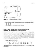
Figure
12.8

Temperature rise
("C)
in substrate, interface layer, and diamond
layer for diamond on
AISI
304
stainless steel with a silicon nitride interface layer.
(U
=
12.7 m/sec,
I
=
0.25 mm.)
Effects
of
Varying Parameters
The effects of varying the sliding velocity of the solid,
U,
and the width of
contact,
I,
are examined in this section. Because the temperature rise in an
uncoated substrate is inversely proportional to the square root of the sliding
velocity,
AT
oc
l/m,
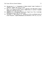
it is expected that the temperature rise for the multi-
layered case will follow suit. Figure
12.9

illustrates this case. The para-
meters, except for
U,
are the same as in Fig.
12.8.
As
would be expected,
the magnitude of the temperature rise for the substrate and layers dropped
with the increase in sliding velocity.
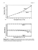
The effect of increasing
I,
the width of contact,
is
now considered.
Because
I
follows the same inverse relationships as
U
for the unlayered
substrate,
AT
a
1/&,
it
is
expected that the magnitude of the temperature
rise will decrease. Figure 12.10 illustrates this case. The parameters, except
for
I,
are the same as in Fig.

12.8.
As
would be expected, the magnitude of
the temperature rise for the substrate and layers dropped with the increase in
contact width.
120
110
100
90
o^
80
O-
0)
70
cn
60
50
a
Ot
-10
1
1
-20
1
I
I
I
I
I
I

I
1
6
8
10 12 14
16
0
2
4
ho,
x
103
Figure
12.9
Temperature rsie
("C)
in substrate, interface layer, and diamond
layer for diamond on
AISI
304
stainless steel with a silicon nitride interface layer
(velocity increase with length of contact constant).
(U
=
50.8 m/sec,
1
=
0.125 mm.)
100
1

I
I
I
I
I I
I
1
90
n
80
Q)
cn
E
70
3
1
60
0)
P
E
50
E
8!
40
30
__
0
2
4
6

8
10
12 14 16
h,,,
x
10'
Figure
12.10
Temperature rise
("C)
in
substrate, interface layer, and diamond
layer for diamond on
AISI
304
stainless steel with a silicon nitride interface layer
(velocity constant with length of contact increase).
(U
=
12.7
m/sec,
I
=
1.375
mm.)
48
I
482
Chapter
I2

12.8
THERMAL
STRESS
CONSIDERATIONS
In this section, simplified equations are developed for predicting the magni-
tude
of
the thermal stresses in a multilayered coating. The thermal stress in
the substrate will
be
combined with the contact stress to determine a max-
imum stress value for calculating a life debit due to thermal fatigue.
12.8.1 Thermal Stress Relationships
Nominal stress relationships for design purposes developed in the following
sections refer to the diagram in Fig.
12.1
1.
This figure defines the variables
used in predicting normal and shear thermal stresses for the case of a multi-
layer semi-infinite substrate moving under a stationary heat source with a
Hertzian distribution.
12.8.2 Normal Stresses
The
“normal” thermal stress in an axial beam built in at both ends
is
proportional to the increase in temperature and can be expected as:
t~
=
EcYAT
(1

2.7)
Figure
12.1
1
Model used in calculating thermal stress in multilayer coatings.
Surface
Coating
483
If this equation is used for a simplified model, then we have the following
equation to describe the normal stress in the diamond, interface coating, and
substrate:
(1
2.8)
where
Td,
TK,
and
ry.y
are the temperature differentials between each
of
the
layers and its substrate. Note that
Eq.
(12.8)
is a nominal relationship for
design approximation only.
12.8.3 Shear Stresses
Shear stress can be determined by dividing the shear force,
F,,
by the shear

area,
A,y.
The shear force can be approximated by the difference in normal
stresses between two layers times the cross-sectional area
of
Fy
=
(02
-
ol)A,
The shear stress can now be written
as
(
12.9)
Now, referring to Fig.
12.1
1,
if we substitute
A,.
=
/I,
and
A,y
=
/m,
we have:
h
I
t
=

(a2
-
01)
-
(
12.10)
and can write the following simplified equations for the shear stress between
the diamond and interface layers, and the interface layer and the substrate:
h.
,
I
tyis
=
(ass
-
ag)
rJ
(12.1
1)
Figures 12.12 and
12.13
show the calculated nominal thermal stresses and
interface shear stresses for the examples considered in the previous sections
using equal thickness layers
of
silicon nitride and diamond on stainless steel.
12.8.4 Life Improvement Due to Surface Coating
The effect
of
thermal stress on the life of a stainless steel substrate is con-

sidered with and without protective coating. In this example, coating layers
7x1
0'
6x1
0'
5x10'
8
4x10'
v)
3
3x10'
0
5
3
E
2x10'
1
xl
0'
0
0
Figure
1
2.1 2
interface layer.
nitride. Note:
1
=
0.25mm.)
2 4 6

8
10 12 14 16
h
x103
0.
Normal stress (Pa) for various thicknesses (mm) of diamond and
Substrate is AISI
304
stainless steel and interface layer is silicon
h.'
I/
=
hd
=
h,,
oI
=
ad,
a2
=
aq
and
a3
=
a.s.s.
(U
=
12.7m/sec,
A
a

a
Y
t
5x1
0'
1
1 1
n.
1
-nu-
$
-1~10'
0)
L:
cn
-a1
0'
-a1
0'
I
-
0
2 4 6
8
10 12 14 16
ho
x103
.
Figure 12.13
Shear stress (Pa) for various thicknesses (mm) of diamond and

interface layer. Substrate is
AISI
304
stainless steel and interface layer is silicon
nitride. Note:
h,
=
h,l
=
h,,
tl
=
rclf, and
r2
=
rif:ss.
(U
=
12.7m/sec,
1
=
0.25mm.)
484
Surface
Coating
485
of
diamond and silicon nitride of equal thickness are used as in the previous
case. The Hertzian contact stress is combined with the thermal stress using
the Von Mises distortion energy theory for predicting the relative surface

damage. The results for different coating thicknesses are given in Fig.
12.14
as an illustration. It can be seen from the figure that considerable improve-
ment in life can be expected as a result of the coating. The improvement
tends towards an asymptotic value for relatively thick layers.
10’
1
OS
1
0’
0
2
4
6
8
10
12 14
16
h
x10’
0”
Figure
12.14
Life improvement in cycles versus thickness of diamond film in
mm. Substrate is AISI
304
stainless steel and interface layer is silicon nitride.
Note:
hjf
=

hd
=
h,
and contact stress level is
1000
MPa.
(U
=
12.7m/sec,
1
=
0.25mm.)
REFERENCES
1.
Bhushan,
B.,
and Gupta, B.
K.,
Handbook
of
Tribology, McGraw-Hill, New
York, NY, 1991.
2. Sherbiney, M. A., and Halling,
J.,
“Friction and Wear of Ion-Plated Soft
Metallic Films,” Wear, 1977, Vol.
45,
pp. 21
1-220.
Chapter

I2
486
3.
4.
5.
6.
7.
8.
9.
10.
11.
Yoder,
M.,
“Diamond Properties and Applications,” Diamond Films and
Coating: Development, Properties, and Application, Davis, R. (Ed.), Park
Ridge, NJ, Noyes Publications, 1993, pp. 1-30.
Spear,
K.,
and Dismukes, J. (Eds), Synthetic Diamond: Emerging CVD Science
and Technology, John Wiley
&
Sons, New York, NY, 1994, p. 663.
Field, J. (Ed.), The Properties of Natural and Synthetic Diamond, Academic
Press/Harcourt Brace Jovanovich, London, England, 1992.
Singh, R., Private communications, Dept. of Material Science, Univ. of
Florida-GainesviIle.
Busch, J., and Dismukes, J., “A Comparative Assessment of CVD Diamond
Manufacturing Technology and Economics,” Synthetic Diamond: Emerging
CVD Science and Technology, Spear,
K.

and Dismukes, J. (Eds), John Wiley
&
Sons, New York, NY, 1994, pp. 581624.
Moustakas, T., “Growth of Diamond by CVD Methods and Effects of Process
Parameters,” Synthetic Diamond: Emerging CVD Science and Technology,
Spear,
K.
and Dismukes, J. (eds), John Wiley
&
Sons, New York, NY, 1994,
Holmberg,
K.,
Ronkainen, H., and Matthews, A., “Wear Mechanisms
of
Coated Sliding Surfaces,” Thin Films in Tribology, Dowson, D., et al. (Eds),
Elsevier Science Publishers B.V., Amsterdam, The Netherlands, 1993, pp. 399-
407.
Matthews, A., Holmberg,
K.,
and Franklin,
S.,
“A Methodology for Coating
Selection,” Thin Films in Tribology, Dowson, D., et al. (Eds), Elsevier Science
Publishers B.V., Amsterdam, The Netherlands, 1993, pp. 429-439.
Rashid, M., and Seireg, A., “Heat Partition and Transient Temperature
Distribution in Layered Concentrated Contacts. Part
I1
-
Dimensionless
Relationships and Numerical Results,” ASME J. Tribol., 1986, pp. 102-107.

pp. 145-192.
FURTHER READING
Coating
Bell, T., “Towards Designer Surfaces,” Met. Mater., August 1991, Vol. 7(8), pp.
478485.
Gao, R., Bai, C.,
Xu,
K.,
and He, J., “Bonding Strength
of
Films Under Cyclic
Loading,” Surface Engineering Volume
11:
Engineering Applications, Dotta, P.
K.
et al. (eds), Royal Society of Chemistry, Cambridge, England, 1992.
Mort, J., “Diamond and Diamond-like Coatings,” Mater. Des., June 1990, Vol.
Rickerby, D.
S.,
and Matthews, A., Advanced Surface Coatings: A Handbook of
Surface Engineering, Blackie and Son, New York, NY, 1991.
Sander, H., and Petersohn, D., “Friction and Wear Behavior
of
PVD-coated
Tribosystems,” Thin Films in Tribology, Dowson, D. et al. (Eds), Elsevier
Science Publishers B.V., Amsterdam, The Netherlands, 1993, pp. 483493.
11(3), pp. 115-121.
Surface
Coating
48

7
Stafford,
K.
N., Subramanian, C., and Wilkes, T. P., “Characterization and Quality
Assurance of Advanced Coatings,” Surface Engineering Volume
11:
Engineering
Applications, Dotta, P.
K.
et al. (Eds), Royal Society of Chemistry, Cambridge,
England,
1992.
Coated
Cutting
Tools
Anon, “Cutting Tools as Good as gold,” Metalwork. Prod., July
1983,
Vol.
127(7),
Bhat, D. G., and Woerner, P.
F.,
“Coatings for Cutting Tools,”
J.
Metals, Feb.
1986,
Bollier,
R.
D.,
“Recoating Enhance Resharpening,” Mod. Mach. Shop, March
1986,

Garside,
B.
L.,
“Improvements in Tools and Product Performance Through PVD
Hale, T., and Graham, D., “How Effective Are the Carbide Coatings?” Aust. Mach.
Hatschek, R.
L.,
“Coatings: Revolution in HSS Tools,” Am. Machin., March
1983,
Hewitt, W. R., and Heminover, D., “TiN Coating Benefits Apply to Solid Carbide
Tools Too,” Cutting Tool Eng., Jan Feb.
1986,
Vol.
36(1-2),
pp.
17-18.
Jackson,
D.,
“Coatings: Key Factor in Cutting Tool Performance,” Mach. Tool Blue
Bk., Vol.
81(1),
pp.
62-64.
Kane, G. E., “Modern Trends in Cutting Tools,” Society of Manufacturing
Engineering,
1982,
pp.
54-55.
Kane, G. E., “Modern Trends in Cutting Tools,” Society of Manufacturing
Engineers,

1982,
pp.
82-87.
Podop, M., “Sputter
Ion
Plating
of
Titanium Nitride Coatings for Tooling
Applications,” Indust. Heat., Jan. 1986, Vol.
53( l),
pp.
20-22.
Schintlmeister, W., Wallgram,
W.,
Kanz, J., and Gigl,
K.,
“Cutting Tools Materials
Coated by Chemical Vapor Deposition,” Wear, Dec.
1984,
Vol.
lOO(1-3),
pp.
Walsh, P., and Bell, D. C., “Recoatingr
A
Viable Option of TIN Coating for Special
Tooling Applications,” Cutting
Tool
Eng., Feb.
1986,
Vol. 38(1), pp.

25-27.
Wick, C., “Coated Carbide Tools Enhance Performance,” Manu. Eng., March
1987,
Wick, C., “HSS Cutting Tools
Gain
a Productivity Edge,” Manuf. Eng., May
1987,
Zichichi, C., “Tool Coatings: Trends and Perspectives,” Carbide Tool J., Jan Feb.
pp.
129-144.
Vol.
38(2),
pp.
68-69.
Vol.
58(10),
pp.
76-81.
Titanium Nitride Process,” Indust. Heat., Vol.
53(9),
pp.
18-20.
Prod. Eng., April
1984,
Vol.
37(4),
pp.
17-19.
Vol.
127(3),

pp.
129-144.
153-1 59.
Vol.
98(3),
pp.
45-50.
Vol.
98(5),
pp.
39-42.
1986,
Vol.
18(1),
pp.
18-20.
13
Some Experimental Studies in Friction,
Lubrication, Wear, and Thermal Shock
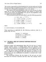
This chapter describes a number of experimental investigations covering
different aspects of tribology. The first set of experiments deals with the
behavior of Hertzian frictional contacts under different types of tangential
loading. In this set, unlubricated spheres pressed against flat surfaces are
subjected to oscillatory loads, impulsive loads, and ramp-type loads respec-
tively.
Another experimental procedure is discussed which can be used to
investigate the oil film pressure generated by a slider with different geome-
tries undergoing a reciprocating motion at a predetermined distance from a
flat surface.
The last two sections describe experimental techniques which can be

used to study the effect of the lubricant properties on surface temperature
and wear in sliding contacts and the effect of repeated thermal shock on the
fatigue life
of
high-carbon steels.
13.1
FRICTIONAL INTERFACE BEHAVIOR
UNDER
SlNUSOlDAL
FORCE EXCITATION
This section describes an experimental technique developed by Seireg and
Weiter
[l]
for studying the vibratory behavior of a ball supported between
two frictional joints. The setup which is utilized in this investigation for
evaluating the “break away” coefficient of friction under sinusoidal tangen-
tial forces is also useful in determining the ball response and the energy
dissipated per cycle under excitations of different amplitudes and frequen-
488
Some Experimental Studies
489
cies. Wear and lubrication studies can be readily performed on different
contact conditions under sinusoidal tangential forces with frequencies
ranging from zero to
2000
Hz and amplitudes from zero to the value neces-
sary to cause gross slip. The main difference between the proposed techni-
que and previous methods is that the tangential force (rather than the
displacement) is sinusoidal and remains as such up to the “break away”
value.

The effect of an oscillating tangential force on the contact surfaces of
elastic bodies has been subject to considerable interest in recent years.
Several valuable contributions are available in the literature. Mindlin
[2]
extended the classical Hertz theory of contact to include the effect of an
increasing tangential force with the normal force unchanged. He predicted
that slip would occur at the edges
of
the contact area and progress inwards
as the tangential force increases. This slip would occur only on annular ring
surfaces. At any point on the contact surface where slip has just taken place,
the tangential component of traction has the same sense as that of the slip,
and its magnitude is equal to the product of a constant coefficient of friction
and the normal component of the pressure at that point. The tractions on
and the displacements of the portion of the contact surface where no slip
occurs are obtained from the solution of the boundary value problem.
Expressions for calculating the relative tangential displacement of distant
points
on
opposite sides of the contact due to a tangential force smaller or
equal to that necessary for gross
slip
are given in Chapter
3.
The theory was
further extended to calculate the displacement due to an oscillating tangen-
tial force within the region of no gross slip. The result is a hysteresis loop
and the energy dissipation for the cycle due to friction can readily be calcu-
lated. Mindlin et al.
[3]

found from experiments on polished crown glass
lenses that the area of the loop at low loads varied as the square of the
displacement, whereas the theory predicts a cube law. The agreement with
the theory was good for large displacements. The oscillating force in their
test was obtained by utilizing a hollow cylinder of barium titanate for the
driving transducer, which is essentially a displacement generator producing
sinusoidal tangential displacement. The force was measured by a disk of
barium titanate cemented between the driving transducer and the sphere.
Johnson
[4]
utilized a torsional pendulum
to
apply the tangential force on
three unlubricated hard steel
balls
on
hard steel flats under a range of
normal loads. Johnson measured the displacements due to static and oscil-
lating tangential forces within the no-gross-slip region. His findings were in
general agreement with the previous work. Goodman and Bowie
[5]
used an
apparatus similar to that of Ref.
3
to study the damping effects at the
contacts of a 1/2 in. diameter stainless steel sphere pressed between two
1/2 in. square by 1/4 in. thick stainless steel plates. The dynamic hysteresis
490
Chapter
13

loops determined in their tests have been shown to conform to the shape
predicted by Mindlin’s theory. Their results of a dimensionless energy dis-
sipation versus the ratio of peak-to-peak displacement at gross slip were in
fair agreement with the theory.
Klint
[6]
studied the effects of oscillating tangential forces within the
region
of
no gross slip on cylindrical specimens in contact.
A
horizontal test
cylinder of 1/8 in. radius is attached to the piston of a hydraulic cylinder and
is forced by the oil pressure against a vertical test cylinder attached to the
table of a shaker producing smooth sinusoidal movements. The hydraulic
cylinder and consequently the horizontal test cylinder, although spring
mounted on the shake table, are essentially fixed in space due to the vibra-
tory characteristic of their support.
A
barium titanate force gage was used between the test specimen and
the shake table. The tangential compliance and the energy dissipation per
cycle were studied for different combinations of materials.
A
region within the no-gross-slip region was found where the displace-
ments are primarily elastic and was defined by the “limit of elastic behavior’.
The coefficient of friction was calculated from the friction force represented
by the flat portion of the force-time relation. Wear and surface damage
conditions were also investigated in the test.
In all the previous experimental procedures, the oscillating tangential
force was provided by applying sinusoidal relative tangential displacements

to the bodies in contact. The force wave forms appear sinusoidal at dis-
placements well below gross slip and then progressively change toward
waves with flat tops as the peak displacement is increased.
The investigation described in this section was, therefore, planned to
provide a sinusoidally changing tangential force with amplitudes up to the
gross slip force, and to study its effects on a sphere pressed between two
flat surfaces by a constant normal force. With such a system, it would be
possible to study the motion of the ball as a mass supported by a non-
conservative hysteretic spring and subjected to sinusoidal excitations (refer
to Fig. 13.1).
13.1.1
Experimental Setup
The apparatus is illustrated diagrammatically in Fig. 13.2. The main test
fixture consists of a
1:
in. ball (a) supported between the flat surfaces of two
cylindrical pins
0.572
in. in diameter. One of the pins
(b)
can be fixed rigidly
to the aluminum frame (c) while the other pin (d) acts as a piston in a brass
air cylinder (e) attached to the frame to provide the normal force. The air
cylinder pressure is controlled by a pressure regulator
(f)
connected to a 150
psi air supply. When the ball is in place, the pins extend
1/16
in. from the
Some Experimental Studies

491
Figure
13.1
tory system.
Diagrammatic representation of (a) forces
on
the ball;
(b)
the vibra-
frame in order to insure maximum rigidity. The test fixture
is
rigidly
fastened to the table (8) of a
50
lbf,
0-2000
Hz
electromagnetic shaker.
A
differential transformer type displacement transducer (h) is rigidly
mounted on the frame with the movable core in contact with the ball and
exerting a
12
gf preload. The transducer excitation and amplification is
carrier
AmplHior
B
H
0
Figure

1
3.2
Diagrammatic representation of the experimental setup.
492 Chapter
13
provided by a
2400
Hz carrier preamplifier.
A
power amplifier is utilized to
provide the input for a direct-writing oscillograph for low-frequency test
recording. A multichannel high-frequency recorder and an oscilloscope
were used for high-frequency measurements. The displacement transducer
has a sensitivity of
1
pm and a range of f0.050in.
An accelerometer (i) is fastened to the shake table to provide a measure
of the acceleration and the resulting dynamic tangential force on the ball. A
power supply and amplifiers provide the input to either recorder or oscillo-
scope. As such, the oscillograph record provides a simultaneous recording of
relative ball displacement and tangential force on the ball. The oscilloscope
can be used to monitor either signal. Or, by utilizing both the
x
and
y
inputs,
a hysteresis loop
is
obtained.
In addition, the output from the calibrated velocity transducer on the

shaker can be used to check the accelerometer calibration.
The shaker frequency and amplitude are controlled by the shaker con-
trol console
(j).
A variable speed motor drive and pulleys (k) are connected
to the control console to provide a predetermined rate of increase for the
shake table amplitude.
13.1.2
Test Procedure
Preparation
of
Test Specimens
The material combinations studied in this test are:
Steel ball on steel pins
Steel ball on brass pins
Brass ball on steel pins
Brass ball on brass pins
The material specifications and surface finish data are given in Table 13.1.
Two lubricants were used in this test. The first is methyl alcohol. The second
is a mild, extreme pressure oil with additives. Viscosity is
SUS
900
to 1000 at
Table
13.1
Test Materials
Hardness Surface roughness
Test specimen (Rockwell
C)
rms (pin.)

Steel
ball
Brass
ball
Steel pin
Brass pin
66
28
65
14
2
4
2
I
.5
Some Experimental Studies
493
100°F. The preparation of the test surfaces is done as follows. The balls are
first cleaned with methyl alcohol and paper towels. The oil is applied to the
surface by wiping with a clean, predipped cloth. The alcohol is applied by
simply dipping the ball (after cleaning) into the alcohol and allowing
it
to
dry in the atmosphere. Throughout this process, the ball is handled using a
plastic holder for each contaminating liquid.
The pins are prepared for each test by finishing their test surfaces with
4/9
sandpaper. The cleaning and surface lubrication is done in the same
manner as for the balls.
13.1.3 Placement of the Specimens

The pins are first placed in the test frame and the ball is then positioned
between them by means of a special fixture. The fixture is designed such as
when the ball is in location, the contacts are along the central axis of the
pins. The stem of the differential transformer will also be touching the ball
at the highest point and will be at its null position. The pin (b) is then fixed
in place by setscrews and the air pressure is applied on pin (d). The posi-
tioning fixture is then withdrawn. The ball is left in position for
3
min before
running each test.
13.1.4 Static Tests
Static tests were performed to calibrate the normal force and to evaluate a
static coefficient of friction. The normal force versus air pressure calibration
was done by means of a scale against the movable pin.
For the static friction tests, the specimens are placed in position and
the pressure adjusted for a certain normal force. The tangential force is
applied at the lowest point of the ball in line with the displacement trans-
ducer. The load is increased successively until gross slip is observed by
watching the indicator on the transducer bridge unit. The test is repeated
four times for each condition.
A
mercury manometer is also used for the
determination
of
the minimum air pressure required to hold the ball in
place when
no
external tangential forces are applied. In this case, the only
acting tangential forces are the ball weight and the spring force from the
transducer. In this test, a relatively high pressure is applied after the speci-

mens are in position. The pressure is then allowed to leak out slowly. The
manometer reading is taken when gross slip is indicated on the meter of
the bridge unit.
494
Chapter
13
13.1.5
Dynamic
Tests
The frame is fastened rigidly to the shaker table and the test specimens are
placed in the frame. The frequency is adjusted to the required value and the
switch on both the recorder and the driving motor (m) is turned on. When
the ball displacement trace on the recorder (or the displacement signal on
the meter of the bridge unit) indicates gross slip, the motor is switched
off
and then reversed to stop the shaker. The dynamic tests were repeated 10
times for each condition and a calibration for the accelerometer is run on the
same chart. The dynamic setup was checked to ensure that no structural
resonance or frequency response existed in the frequency range considered
in the test and that the movable pin had no relative motion with respect to
the frame.
13.1.6
Discussion
of
the
Results
Typical oscillograph records of the ball acceleration and displacement are
shown in Fig. 13.3. A typical plot of the test results
is
shown in Fig. 13.4,

and the coefficients of friction are given in Table 13.2.
The lines representing the relation between the amplitude
T+
of the
tangential force versus the air pressure and normal force
N
were found to
fit both the dynamic data and the static data. For all the tests performed in
this investigation, there was no evidence
of
any difference between the sta-
tically determined coefficient of friction and that determined by dynamic
tests. Gross slip occurred when the tangential force reached the value
required to overcome the static friction. This always happened when the
ball was at the lowest position of its motion or when the total tangential
force was at its maximum value. This can be easily seen in Fig. 13.3b,
representing a magnified ball displacement trace.
A series of tests was run for steel balls on steel pins (with oil contam-
ination) for frequencies between 10 and
500Hz.
No
frequency effects were
observed for this range (refer to Fig. 13.5).
The normal load and consequently the contact stresses and contact area
had no obvious effect on the coefficient of friction. The maximum Hertzian
contact stress at 40
psi
pressure is 105,000 psi for steel on steel, 82,500 psi for
steel on brass, and
69,000

psi for brass on brass.
There was also little difference observed in the coefficient of friction
between the same specimens when tested with either of the used contam-
inating liquids.
Ball vibration relative to the pins could be easily measured and
recorded. An oscillograph trace is shown in Fig. 13.3. Hysteresis loops
495
Figure
13.3
eration:
(a)
slow
speed;
(b)
high
speed.
Recorder
traces
for
reiative
ball displacement
and
shake
table
accel-
representing the sinusoidal tangential force versus ball displacement (rela-
tive to the
pins)
were
also obtained on the scope screen.

Wear patterns, scars, and weldments (especially for clean surfxes
at
high frequencies) were observed. In
cases
when welding occurred very high
tangential forces were required to
break
the frictional joint.
It
was
also
observed
that
when twisting
of
the ball occurred during the
withdrawal of
the
positioning fixture,
a
relatively higher coefficient
of
fric-
496
Chapter
I3
Figure
13.4
Brass ball on steel pins: (a) alcohol lubrication; (b) oil lubrication.
tion existed. This is in accordance with the observations reported by Mason

[7]
and Anderson
[8].
Several tests were run to study the effect of the number of cycles at force
amplitudes lower than required for gross slip. The shaker frequency was
fixed and the amplitude of its vibration was increased in steps. The vibration
was allowed to continue for
5
min at each step.
Gross
slip occurred at the
expected value with no obvious effects due to the load history.
Some Experimental Studies
497
Table
13.2
Coefficients of Friction
Materials
Coefficient of
Ball Pin Lubricant friction
(I)
Steel
Steel
Brass
Brass
S
tee1
Brass
Steel
Brass

Oil
Alcohol
Oil
Alcohol
Oil
Alcohol
Oil
Alcohol
0.09
0.09
0.104
0.1 10
0.105
0.105
0.120
0.121
13.2
FRICTION UNDER IMPULSIVE LOADING
There is considerable practical interest in determining the frictional resis-
tance under impulsive loading. Gaylord and Shu
[9]
reported that some
materials (steel on steel and titanium on steel) exhibited higher static coeffi-
cients of friction under statically applied loads than under shock loads. In
0.0
I
I
I
I
I

I
II
0
40
loo
200
300
400
500
Shake Table Frequency,
f
(Hz)
Figure
13.5
Sample of results of test on frequency effect. Steel on steel
with
oil
lubrication.
their test. the specimen rested
on
an inclined plane. The
load
is applied by
dropping
a
weight
on
to cushioned stops which are attached
to
the loading

rod.
The
study described in this section
[lO]
utilizes the same fixture used in
the previous section
[I]
to
investigate the frictional behavior
of
circular
contacts under the influence of pulse-type loading. The test arrangement
consists of
a
hall
suspended between
two
flat surfiices (Hertzian contacts)
with the impulse load provided by
a
spherical ball suspended as
a
ballistic
pendulum.
13.2.1
Experimental
Arrangement
The appratus used
in
this investigation is represented schematically

in
Fig.
13.6.
The
1:
in.
ball
(a),
is suspended between two cylindrical steel
pins
with
parallel flat ends. One
of
the pins
(b),
is
rigidly attached
to
the frame (c).
while the other pin
(d).
acts
as
an
air
piston
in a precision bore in the fixture
to
provide the normal force. The magnitude
of

the normal force is
a
func-
tion of the regulated air pressure from
a
1000
psi source
(e).
The test fixture
is
rigidly fastened
to
a
steel base
(0.
Figure
I
3.6
Diagramilia
tic
representation
of
the
test
apparatus.
Some Experimental Studies
499
A steel ball (g), 1/2 in. in diameter is cemented to a fine thread and
suspended as shown in Fig. 13.6 to form an
87.3

in. pendulum. This suspen-
sion insures the fall and rebound
of
the ball to be in the same plane. The
initial and final position (after rebound) of the pendulum can be read on a
graduated arc (h), giving accurate indication on the velocity of the impact
ball before and after impact. The velocity ranged between
1
in./sec and
120 in./sec.
The displacement of the ball is measured by means of a differential
transformer type displacement transducer
(i),
rigidly mounted on the
frame with the movable core in contact with the ball (a), with a 12gf
preload. The transducer excitation (2400 Hz) and signal amplification is
provided by a carrier-type preamplifier coupled to a power amplifier
which provides the input to a direct writing oscillograph. The record is
calibrated to give the final ball displacement a
1
pin. sensitivity.
Accurate alignment is provided
so
that the impact between the two
spheres is on the same axis as the displacement transducer.
13.2.2
Test Procedure
The surface preparation consisted
of
washing all contacting surfaces of the

balls and pins with methyl alcohol. The pins are placed in the frame and the
test ball is positioned between the pins by means of the special fixture used in
the previous section to insure proper axial location. The air pressure is then
applied to provide the desired normal force.
The striking ball is held at the required position on the graduated arc by
means
of
a clean steel bar. The ball
is
released by rapidly withdrawing the
bar forward and away in such a manner as to not interfere with the free fall
of the ball. The rebound
of
the ball is then measured on the graduated arc by
observing the maximum position
of
the ball after impact. The displacement
of the ball for each drop (impact)
is
detected by the transducer and
recorded,
13.2.3
Theory
The pulse characteristics in this investigation are calculated by means of the
Hertz theory
of
impact
[I
1,
121. The theory treats the impact of two spheres

as a statical problem and takes no consideration to the dissipation of energy
during the impact. The result, although both static and elastic in nature, has
been widely applied to impact situations where permanent deformations
were produced. The application of Hertz theory beyond the limits of its
validity has been justified on the basis that it appears to predict accurately
most of the impact parameters that can be experimentally verified.
In
the
500
Chapter
13
case of central impact of two stainless steel spheres with
1/2
in. and
1
in.
diameter, respectively, the Hertz theory gives the following expressions for
the maximum force and duration of impact:
Fmax
=
1.665~'.~
Ibf
98
x
10-6
u1/5
sec
t=
where
v

=
velocity
of
approach
(in./sec)
The conservation of momentum and restitution equations for the system
under consideration can be written as:
and
from which
and
(13.1)
The velocity of the struck ball,
yf,
after impact can also be expressed in
terms of the impact velocity,
wf,
as:
v(1
+e)
1
+-
ml
Vf
=
(1
3.2)
The ratio
v,/v
of the striking ball under consideration for the different
conditions of impact was determined experimentally by reading the angles

of drop and rebound of the pendulum. It was found to be
w,/v=O.83
throughout the test.
Some Experimental Studies
501
Substitution in Eq. (13.1) gives
e
=
0.949.
Equation (13.2) therefore
gives:
VJ
=
(0.1 171)~
(1
3.3)
The kinetic energy of the struck ball due to the impact is:
fm2$
=
i(7.4
x
10-4(0.1 171)2~2
=
5.075
x
10-6~2
(1
3.4)
This energy represents the area under the frictional force-displacement
curve up to the peak displacement. The minimum impact energy necessary

for gross slip is given by
where
is the area under the friction force displacement curve up to gross slip and
C
=
factor compensating for the nonlinearity
of
the force-displacement
relationship.
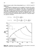
A
dimensionless friction force-displacement curve is plotted in Fig. 13.7
according
to
Mindlin’s theory. The graph shows
F/Fo
versus
6/J0
as
represented by
(1
3.6)
k,
is also calculated for the case under consideration:
k,
=
2.27
x
105(N)’/2
(1
3.7)

and
C,
which is a dimensionless factor defined by Eq. (13.5)’ is found from
Fig. 13.7 as
Area onabo
Area oabo
c=
=
1.228
(1
3.8)
Because there is no way to detect gross slip in this investigation except by
means of the permanent displacement of the ball, Mindlin’s theory is again
utilized to calculate this value. This permanent displacement within the
region of no gross slip is given by:
502
Chapter
13
616,
Figure
13.7
(Mindlin's theory).
Dimensionless displacement
of
ball within the region
of
no gross slip
For
gross slip
F/Fo

=
1
and substitution in
Eq.
(13.9)
gives:
d0
-
=
0.26
60
In
this case:
which can be written as:
5.075~~
-
0.1
392(N)'j36;
2N(d
-
O.26aO)
pk
=
(1
3.9)
(13.10)
(13.12)
Some Experiment
a1
Studies

503
or in the form:
(13.13)
5.075~~
-
0.1392(N)''36%
+
0.52pkN60
d=
2pkN
Equations
(13.11), (13.12),
and
(13.13)
are utilized for evaluation
of
the
frictional characteristics of the joint from the experimental data as explained
in the following.
13.2.4
Discussion
of
Results
Figure
13.8
shows a plot of the permanent ball displacement d(pin.) versus
the striker velocity v(in./sec) for low values of impact under various normal
forces. Equation
(13.11)
representing the conditions for gross slip is also

plotted on the graph. The intersection of these lines
for
each normal force
with the corresponding experimental curve gives permanent displacement
(4)
and the striker velocity
(vo)
at gross slip. The peak displacement
a0
for
gross slip can therefore be obtained
from
the equation:
0
5
10
15
20
25
Velocity
&Approach,
V
(id8)
Figure
13.8
Evaluation
of
conditions
at
gross

slip.
504
do
*
So
=
-
in.
0.26
Chapter
13
and the tangential force for gross slip is therefore:
from which the coefficient of friction for gross slip is:
F~
2.27
105~113
d0
p,.
-
-
=
60
=
0.437
-
'-2N 2N N2/3
(1
3.14)
By substituting the value of
do

from Fig. 13.8 in Eq. (13.14) the coefficient of
friction for gross slip is readily calculated. They are plotted versus the striker
velocity in Fig. 13.9. The average value for this coefficient is found to be
p,
=
0.305.
Equation (1 3.12) is now used to calculate the kinetic coefficient of fric-
tion
pk
(the average value of the coefficient of friction during slip). For any
particular normal force, the value of
60
at gross slip is substituted in the
equation. Values of
v
in the region beyond gross slip and the corresponding
0.3
1
0.0
1 10
1
00
Velocity
of
Approach, V(in/s)
500
Figure
13.9
Values
of

static and kinetic coefficients
of
friction.
x,
N
=
15.25
lb;
A,
N
=
30.51b;
0,
N
=
45.751b;
0,
N
=
61.01b;
+,
N
=
91.51b.