Friction and Lubrication in Mechanical Design Episode 2 Part 12 pdf

Some
Experimental
Studies
505
values of
d
are then used to calculate
&.
This kinetic coefficient of friction is
also plotted against the striker velocity
U
in Fig. 13.9. Its value
is
found to be
&
=
0.22
and is independent
of
the normal force.
Equation (13.13)
is
then used to obtain a theoretical plot of
d
versus
U
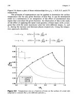
beyond gross slip. This is shown by the solid lines in Fig. 13.10. The correla-
tion between the calculated curves and the experimental data is evident.
The peak force and the time duration of the impact corresponding
to
gross slip are listed in Table 13.3 as a function of the normal force.

It
can be
‘oooo
m
1
2
4
6
8
10
20
40
60
80100 150200
Velocity
of
Approach,
V
(ink)
Figure
13.10
Ball displacement
for
impacts causing gross slip. (From
Ref.
10.)
506
Chapter
13
Table

13.3
Pulse
Characteristics
N
(Ib)
vo
(in./sec)
U:’
Knax
(W
t
(CLW
~~
15.25 4.35 5.75
1.321 9.57
74.1
30.5 7.75 11.7
1.511
19.47 64.8
45.75 10.95 17.5
1.600
29.10 61.2
61.0 13.4 22.6
1.686 37.6
58.8
91.5
18.7
34.0 1.818
55.6 53.9
easily seen that the coefficient of static friction based on the peak of the

Hertzian pulse checks very closely with the value obtained from energy
consideration. It should be noted here, however, that the pulse duration
in this investigation varies between 0.35r, and 0.36r,, where r, is the equi-
valent natural period of the ball suspended on the frictional support, as
calculated from:
At this ratio of pulse duration to natural frequency, the shape of the pulse is
not
of
significant value and the transient response of the system is the same
as the static response to the pulse within the range of this test [13].
It is interesting to note that the gross slip coefficient of friction under
impulsive loading is equal to 0.305 for the materials used and is independent
of the normal load for the range investigated. This is more than three times
higher than the corresponding value under static or vibrating loads.
The experimental results also show that at gross slip, the frictional joint
undergoes a sudden drop in frictional resistance. The frictional resistance in
the gross slip region is substantially constant and corresponds to
&
=
0.22.
All the energy applied during gross slip is dissipated.
Figure 13.1
1
represents a dimensionless frictional force versus displace-
ment plot which was found to be descriptive of the behavior of frictional
contacts under impulsive loading.
13.3
VISCOELASTIC BEHAVIOR
OF
FRICTIONAL HERTZIAN

CONTACTS
UNDER
RAMP-TYPE
LOADS
It has been observed during the tests described in the previous section, that
considerable slip of a “creep” nature may occur under sustained loads with
Some Experimental Studies
507
Figure
13.1
1
impulsive loading.
Representation
of
frictional behavior
of
Hertzian contacts under
values below those necessary to produce ball accelerations which character-
ize gross slip under such conditions.
A
phenomenon of “creep” in the frictional contact between a hemi-
sphere of lead and glass flats was detected by Parker and Hatch
[14]
during
their studies on the nature of static friction. Similar observations were also
reported by Bristow
[15].
The investigation described in this section, was therefore undertaken to
study this “creep” phenomenon in the region below gross slip in static
friction tests when the tangential loads are applied at relatively low rates

and allowed to dwell for relatively short periods. The utilized specimens and
surface conditions are the same as those tested previously under vibratory
and impulsive loads
[
161.
13.3.1
Experimental Arrangement
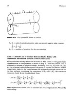
The apparatus used in this investigation is schematically represented in Fig.
13.12.
A
lf in. diameter steel ball (a) is suspended between the two parallel
flat surfaces of two identical hear steel inserts (b),
(c).
Insert (b) is fastened to
a rigid steel frame
(d),
whereas (c) is fastened to a solid steel block (e) which
can slide tightly with minimum friction in the frame under the influence of
air pressure acting on a flexible diaphragm
(f).
The air pressure is controlled
508
Chapter
13
Figure
13.1
2
Diagrammatic representation
of
the test arrangement.

by a regulator and measured by means of a mercury manometer (g).
Calibration of the normal force applied on the ball versus manometer read-
ing is checked periodically by replacing the ball by a ring-type strain gage
force meter of
14
in. outer diameter. The tangential load on the ball is
applied by a special loading device capable of different rates of load appli-
cation ranging from 0.12251b/sec to more than ten times this value. The
device is composed of a lever (1) carrying a known weight
(w)
which can be
moved on the lever by means of a string on a rotating drum. The rotation
of
the drum is controlled by pulleys driven by a variable-speed motor. The
position of the weight from the center of the lever is indicative of the tan-
gential force on the ball. This can be easily detected by the rotation of the
drum.
A
variable resistance (r) connected to the drum was used in conjunc-
tion with a
6V
DC battery to produce a volage which is calibrated to
indicate the tangential force on the ball. The calibration was done by utiliz-
ing the ring-type strain gage force meter.
The tangential force can be either applied to the ball or to the frame at
the inserts by removing or inserting a pin
(p)
which disengages a special fork
(h) to apply the load to the ball or to the frame, respectively. This arrange-
ment makes

it
convenient to evaluate the apparatus deformations and hys-
teresis under any particular test condition before applying the tangential
Some Experimental Studies
509
load. The ball displacement is measured by a differential transformer-type
displacement transducer (t) rigidly fastened to the frame with the movable
core in contact with the ball under a
12
g
preload. The transducer excitation
and signal amplification is provided by a carrier-type preamplifier
(s)
coupled to a power amplifier which provides the input to the
x-y
plotters
Accurate alignment is provided, ensuring that the load on the sphere is
on the same axis as the displacement transducer. The whole apparatus
is
enclosed in a plastic box (n) which is thermostatically controlled to within
f1”F.
Two
x-y
plotters were used simultaneously to record the load-displace-
ment and the displacement-time behavior of the ball under different load
(41
7
42).
regimes.
As a general procedure, the apparatus was subjected to two consecutive

hysteresis loops corresponding to the highest level of tangential load in all
tests (approximately 121b).
A
third load cycle, similar to the expected fric-
tional cycle, was applied to the apparatus and recorded. This cycle was
found to give a reproducible hysteresis loop for the apparatus itself. The
pin (p) was withdrawn from the loading fork
(h)
and the particular load
regime is then applied to the ball.
The following are samples of the tests performed in this investigation. In
the test illustrated in Fig. 13.13a, the ball was subjected to a
2
min dwell at a
load level
of
approximately
0.87
the gross slip value. The load was then
released and reapplied until gross slip occurred. The loading, unloading, and
reloading up to gross slip were performed at the same rate. The ball was
repositioned and subjected to six successive hysteresis loops after a repro-
ducible apparatus loop was obtained. In the seventh loop the load was again
sustained for 2 min at
0.87
the gross slip value, after which the load was
released and reapplied until gross slip occurred. The figure shows strain-
hardening effects in the successive loops with no significant change in the
“creep” displacement during the
2 min dwell.

As
shown in Fig. 13.13b, the
2
min dwell tests were also performed at
different load levels. In each of the these tests, the load was sustained after
two successive load cycles. The load was released at the same rate, after which
the ball was loaded to gross slip. The data show an exponential increase in the
creep displacement as the dwell load approaches the gross slip value.
Figure 13.13~ shows typical results from tests where the ball was sub-
jected to several successive 2 rnin dwell cycles. It can be seen that the “creep”
displacement diminished with successive cycles. The decay rate was found to
be more pronounced in the early cycles.
Figure 13.14 shows typical time-displacement tests in which the load
was applied at the particular rate and allowed to dwell at different points
t
Figure
13.1
3
(a) Load-displacement curves with
18.5
lbf normal force.
(b)
Frictional loops at different load levels with 301b normal force. (c) Successive
dwell loops at the same load level with
50
lb normal force.
A:
reproducible apparatus
loop; B: frictional hysteresis loops (zero dwell);
C:

frictional hysteresis loops
(2
min
dwell);
D:
final frictional tests carried to gross slip. (Force scale:
1
unit
=
1.681bf.
Ball displacement: pin.)
510
Some Experiment
a1
Studies
51
I
7
DbpIacament
Scab
(in)
-
012846
Loading
Rata
-
0.12261bf/s
SeCOndr
111111111111111111111
(a)

Time
(8)
4
-
012a4s
second8
Loading
Rate
0.42
Ibfh
I1111
IIIIIII
3
Figure
13.1
4
Displacement-time curves for
30
lb normal load. (a)
0.1225
lb/sec
loading rate; (b)
0.42
lb/sec loading rate.
512
Chapter
I3
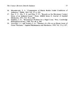
within the region of gross slip. The dependency of the creep displacement on
the rate of ball displacement at the onset of dwell can be readily seen. Figure
13.15 shows the plot of this relationship from the experimental data for

normal loads of
30
and 501b, respectively. The experimental results, as
illustrated by Figs 13.13a and b, indicate that the creep behavior of the
frictional contacts (as in most low-temperature instances of creep) can be
approximated by a Boltzmann model as shown in Figs. 13.16, 13.17, and
13.8.
The creep displacement can, therefore, be represented by
[
17, 181
where
C
is a characteristic constant when a linear model is assumed.
The factor
C
has been evaluated empirically by plotting the slope
(xc)i
of the displacement-time curve at the onset of creep versus the total creep
displacement
X,.
This can be done for any normal load, test temperature,
and rate of load application. Figure 13.15 shows an example of such plots at
80°F
with normal loads of 30 and 501b, respectively. The points represent
data from load application rates of 0.1225, 0.2667, and 0.421b/sec.
The repeated “no-dwell” cycling tests at load levels below gross slip
showed clearly that the largest plastic displacements occurred during the
first cycle. The area of the hysteresis loop diminished progressively with
the number of cycles and the rate of decay of the loop area also decreased
with the number of cycles. Johnson [4] and O’Connor and Johnson [19]

observed the phenomenon and attributed
it
to an increase in the local co-
efficient of friction in the annulus of slip by the fretting action.
These effects were observed by successive 2 min dwell cycles. The tests
also showed no significant dependence of the 2 min creep displacements on
the number of no-dwell cycles which preceded them with the same maximum
load.
Gross slip curves, when produced without previous cycling history,
exhibited considerably higher displacements in the region close to gross
slip than expected by Mindlin’s theory [2, 31. Repeated cycling caused strain
hardening and brought the load4isplacement curves closer to Mindlin’s
prediction.
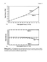
Figure 13.17 shows the deviation of the experimental displacement-time
curves from Mindlin’s theory at the lower loads and the accuracy of the
linear viscoelastic model in describing the creep behavior.
It
should be noted
here that the values of the coefficient of friction at gross lip varied between
0.09 and
0.095
in most of the tests. These values are essentially the same as
those in the previous tests with vibratory loads.
Some Experimental Studies
513
0.0002
n
C
c
Y

5
f
0
P
I
a
I
0.0001
i
1
0
f
a!
al
I
o.Ooo0
I I
0.00000
o.oooo1
O.OOOO2
XI
-
Initial
Cmp
Dlsplrcement
(In)
Figure
13.1
5
Maximum creep versus initial creep rate.

b
a
I
0.00003
Figure
1
3.1
6
Boltzmann model.
0.00015
CI
g
0.00010
U
f
$
0
Q
P
-
0.00005
0.00000
Time
(8)
Figure 13.1
7
time curves.
Comparison between experimental and calculated displacenient-
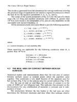
Figure
13.1

8
5
14
Diagrammatic reprcsentation
of
the experimental
setup.
Some Experimental Studies
515
13.4
FILM
PRESSURE
IN
RECIPROCATING
SLIDER
BEARINGS
An experimental procedure for evaluating the oil film pressure in recipro-
cating slider bearings with arbitrary geometry is presented in this section
[20].
A special test fixture is constructed where the slider is inserted in such a
way as to insure that a specific film geometry is achieved and maintained
throughout the test. The pressure is monitored at three different locations
along the central line of the slider by means of miniature pressure transdu-
cers. The setup is capable of producing oscillatory sliding motions with
different strokes and speeds and can
be
used to simulate a variety
of
film
geometries and operating conditions. The results indicate the development

of negative pressure and cavitation during the return stroke. The pressure
distribution during the forward stroke follows the same pattern as that
predicted by isoviscous theory. The magnitude of the pressures, however,
can be higher or lower than the isoviscous values depending on the operat-
ing conditions. The peak pressure during the forward stroke follows a
square root relationship with the instantaneous sliding velocity, which can
be attributed to the thermohydrodynamic phenomenon discussed in
Chapter
6.
13.4.1
Experimental Setup
The experimental setup is diagrammatically represented in Fig. 13.18. The
main components of the setup and
a
brief explanation of their functions are
listed below:
A
shaper carrier is used for providing the reciprocating motion, the
speed and stroke are adjustable.
A
slider block is used for holding the slider in order to maintain the film
geometry constant relative to the sliding surface. The geometry is
illustrated in Fig. 13.19.
A
steel bar is used for transmitting the reciprocating motion from the
carrier to the slider. It also serves as a cantilever spring to force
down the brass surface
of
the slider block against the sliding sur-
face.

The slider surface is a well-ground steel plate. The slider block is sub-
merged in an oil bath. The temperature of the bath is monitored by
a thermometer throughout the test.
A potentiometer is used to record the position of the slider.
A
two-channel oscilloscope is used for monitoring the signals from the
A multichannel chart recorder is used for recording the signals.
pressure transducers.
516
Chapter
13
Figure
13.1
9
Geometry
of
the tapered slider bearing.
Three temperature-compensated strain gauge transducers with a range
The minimum film thickness and slope of the slider is easily adjusted by
changing the metal shims between the slider and the slider block. Three oil
holes of 0.0315 in. diameter, which are located on the slider surface, allow
the transducers to pick up the pressure. The potentiometer is utilized to
provide the information on change of position, and speed as a function of
time. For all the given data, the same film geometry is used with two speeds,
18 and 37 strokes per minute (spm), respectively. The 18 spm produces a
maximum speed of 9.17 in./sec when the slider is moving forward with an
11
in. stroke. The maximum speed corresponding to 37 spm is 18.07 in./sec
with the same stroke. The oil bath temperature was maintained at
25

f
0.5"C.
from
0
to 100 psi are used for pressure sensing.
1
3.4.2
Experimental Results
A
sample of the recorded data is shown in Fig. 13.20. The figure shows the
pressure-position data for the test slider bearing when the
SAE
5
oil is used
at a speed of 18 spm. In this case, the minimum film thickness is
0.006
in.
and the slope is 0.0009in./in.
It
can be seen that for the first stroke, at the second and third oil holes,
an oscillatory pressure drop occurs before the peak pressure is reached.
A
sample of the pressure data from the three transducers
is
given in Table 13.1
Some Experimental Studies
51
7
Fsec
3.10

in
10
psi
f
Figure
13.20
Sample experimental data:
h2
=
0.0006in.,
m
=
0.0009in./in.,
18
spm,
SAE
5
oil,
25°C.
at four different instances in time, as indicated by (a), (b), (c), and (d) in
Fig.
13.20.
The corresponding instantaneous velocities
of
the slider are also
tabulated.
It was noticed during the tests that the peak pressure for each stroke
dropped gradually as the test continued. This can be attributed to the for-
mation of air bubbles which are generated during the backstroke and accu-
mulate inside the tube leading to the pressure transducer. Before each test,

the transducer is filled with
oil
to ensure that there are no bubbles in it. For
the same test conditions, the pressure generated in the first stroke
is
found to
be reproducible, and the peak pressure of that stroke can be used
to
repre-
sent the pressure corresponding to the maximum speed of the slider.
Figures
13.21
and
13.22
show sample results of the pressure distribu-
tions along the central line
of
the slider bearing in the direction of motion.
5
18
30
25
20
=
r)
P
v
2
l5
a

Y)
b
e
10
5
0
Chapter
13
I
1
I
.
I
I
I
I
I
0.00
0.25
0.50 0.75
1
.oo
1.25 1.50
Location
(In)
Figure
13.21
Pressure distribution along the central line in the direction
of
motion:

h2
=
0.0006in.,
rn
=
0.0009in./in.,
V
=
9.17in./sec.,
p
=
31.03
x
10-6
reyn.
The experimental results are compared to those predicted by isothermal
theory, which takes into consideration the temperature rise in the bearing
for the given film geometry, oil, and inlet temperature. It is noticed that the
magnitudes
of
the pressures measured may differ considerably from those
predicted by the isothermal hydrodynamic theory. However, the calculated
and measured pressures retain the same normalized shape for any given film
geometry,
oil,
and sliding speed.
It
is
worth noting that the isothermal theory can either underestimate
(refer to Fig. 13.21) or overestimate the preak pressure (refer to Fig. 13.22).

This has been found to depend on the values
of
minimum film thickness,
viscosity, and speed in a similar maner as discussed in Chapter
6.
Figures
(1
3.23 and 13.24) show the pressure-speed characteristic of test
slider bearings. It can be seen that the pressure is proportional to the square
root
of
the speed as was the case for journal bearings.
Some Experimental Studies
519
80
60
=
Y
B
a
g!
40
g!
p.
20
0
.
I
I
I

I
.
.
I
.
0.00
0.25
0.50
0.75
1
.oo
1.25 1
SO
Location
(in)
Figure
13.22
Pressure distribution along the central line in the direction
of
motion:
h2
=
0.0010in.,
m
=
0.0011 in./in.,
V
=
18.01 in./sec.,
p

=
1.986
x
10-5
reyn.
13.5
EFFECT
OF
LUBRICANT PROPERTIES ON TEMPERATURE
AND
WEAR
IN SLIDING CONCENTRATED CONTACTS
The experimental study discussed in this section deals with investigating the
effect of some of the physical properties of lubricants on the contact tem-
perature and wear in heavily loaded Hertzian contacts under sliding condi-
tions
[21].
The surface temperature and wear in a rotating mild steel shaft
are measured under different loads applied by a tungsten carbide slider. The
carbide tip and the shaft are used as part of a dynamic thermocouple system
to monitor the contact temperature. Tests are conducted for Hertzian pres-
sures ranging from
1250
to
2140
MPa
(1.8
1
x
10’

-
3.10
x
10’
psi) and slid-
ing speeds from
0.4
to
1.3
m/sec
(943-3 142
in./min). Temperature and wear
520
80
60
=
U
8
t
e!
40
3
Y)
Q
20
0
0
Chapter
13
5

10
15
8p.d
(ids)
20
Figure
13.23
Pressure-speed characteristic
of
slider bearing:
h2
=
0.006
in.,
m
=
0.009in./in.,
SAE
5
oil,
25°C.
data are given from tests with a heavy duty
oil
(SAE
80W-90),
a high-
viscosity residual compound, a vegetable oil, and water-miscible cutting
fluid
(0.0476%
emulsifiable

oil
by volume). The results show that, for the
considered tests, viscosity does not appear to be the significant property
of
the lubricant temperature rise and wear rate as indicated by the scar depth
under similar test conditions.
13.5.1
Experimental Setup
The experimental setup used in this study is illustrated diagrammatically in
Fig.
13.25.
The supporting structure consists
of
a steel plate
(I),
pillowblock
(2),
and loading screws
(3).
The rotating shaft
(4)
is supported on bearings
and the desired load is applied on it by the loading screws which are
mounted on the steel plate and apply the load to the pillowblocks. The
Some Experimental Studies
52
I
80
I I
1

60
f
0
0
v
E
40
3
I
3
0
20
0
0
5
10
15
20
SpHd
(in/s)
Figure
13.24
m
=
0.001
1
in./in.,
SAE
20
oil,

25°C.
Pressure-speed characteristic
of
slider bearing:
h2
=
0.0010
in.,
steel plate and the loading screws are electrically insolated from the steel
shaft to reduce possible noise.
A
5 hp variable speed motor
(5)
supplies the power necessary to rotate
the shaft at the desired rotating speed. It has a speed range from 715 to
5000rpm.
A
belt drive
(6)
with a speed ratio 2.4
is
used between the test
shaft and motor, making the range of the test from 300 to 2000rpm.
A
strain gage type load cell
(7)
supports the tungsten carbide tip and
provides a continuous record
of
the load.

A
dynamic thermocouple circuit is used to monitor the contact tem-
perature as shown in Fig.
13.25a
and
illustrated in detail in Fig. 13.25b. The
main junction is the low carbon steel shaft (4)
(AISI
1020) and the tungsten
carbide tip
(8)
(80%
WC,
8%Co).
Junction
X
is
kept at constant tempera-
ture by running cooling water through it, whereas the other
Y,
which has
the least effect on the calibration,
is
kept at room temperature (2Oo-24"C).
Due to the influence of the variable temeprature of junction
Y,
the system
may have an error of approximately 1%.
522
E

Chapter
13
Dynamic
Thermocouple
Junction
Copper
Y,wcron
(slip ring contact point)
Copper
%,,,,,-
(WC-Copper
water
tube)
Figure
1
5.25
(a) Diagrammatic representation
of
the experimental
Thermocouple circuit.
(b)
setup.
(b)
The slip ring
(9)
is used to transmit the thermoelectric signal from the
rotating shaft.
A
two-channel recorder (1)
is

used to simultaneously record the load
and the contact temperature. The latter is calibrated in a bath of the lubri-
cant using a mercury thermometer. The rotational speed of the shaft is
measured by strobe light.
A
lubricant reservoir (1 1) is mounted at a prescribed height above the
test setup. The flow rate of the lubricant is calibrated for the different fluid
levels which are maintained within a certain range throughout each test to
keep the flow rate approximately constant.
Some Experimental Studies
523
13.5.2 Test Specimens
The test specimen is selected as a steel shaft 25mm (1 in.) diameter sup-
ported at a 250mm (loin.) span. The rider is tungsten carbide with a
cylindrical surface 9.5mm (0.37511.) radius and a modulus of elasticity of
55
1.6 MPa
(80
x
106 psi). The length of the shaft allows for several succes-
sive tests to be conveniently run on the same shaft. The flexibility of the
shaft also helps in controlling the applied load and minimizing the load
fluctuation during the rotation of the shaft or as a result of wear.
13.5.3 Test lubricants
Four different types of lubricants were used in the performed experiments.
Two of them represent heavy-duty lubricants, and the others are non-
conventional fluids which are not generally used in common lubrication
practices. The selected lubricants are as follows:
1.
SAE

80W90 oil
2.
A
very-high-viscosity residual compound
3. Water-miscible cutting fluid (0.0476% emulsifiable oil by
volume)
4. Vegetable oil
Lubricants 1,
3,
and 4 were applied at the contact location at different flow
rates varying from 0.35 ml/sec to 2.1 ml/sec. The residual compound was
applied directly on the shaft by
a
brush because
it
is too thick to flow.
Viscosity data at
38°C
(100°F)
for the different lubricants used are as
follows: 200cSt for
SAW
80W90 oil, 583 cSt for the residual compound
0.65 cSt for water, and
40
cSt for the vegetable oil.
13.5.4 Wear Scar Measurement
In all the previous tests, wear scar geometry was measured after the tests
using a Talysuf model 3 (Taylor-Hobson) surface texture measuring
machine.

The shaft is supported on the table by a set of V-blocks in the
machine. The chart recorder is calibrated by using a calibration plate
with certain scar depth. The wear scar is measured at
90"
intervals around
the circumference of the shaft by moving the stylus along the shaft surface
in the axial direction.
524
Chapter
13
13.5.5
Results
Typical data on temperature and wear for different conditions of load and
speed are illustrated in the following. Figure 13.26a shows reuslts from
experiments run with
SAW 80W90
oil lubrication at a particular shaft
speed under 45,
89,
133, and 178
N
(10, 20, 30, and
40
lbf) in succession
without changing the point of load application. The test speeds in this case
are 300,
500,
750, and 1000 rpm. The point of load application is changed
after each constant speed test to a new location on the shaft.
Summary temperature data from the test with residual compound and

water-miscible cutting fluid lubrication are shown in Figs 13.26b and c,
respectively.
Some of the wear scars from the previous tests at 300 and 1000 rpm are
shown in Fig. 13.27. These scars are the result of six repeated applications of
each of the four levels for 15 sec and turning the motor off until the tem-
perature cools back to the ambient temperature. The total test duration
corresponds to each scar is approximately 360sec. The maximum scar
depth data are given in Table 13.4. The depth of the wear scar appears to
reflect the magnitude of the temperature rise in all the performed tests.
400
70
-
150
1.1.1.1".
10
15 20
25
30
35
40
Load
(Ibf)
60
80
100
120
140
160
Figure
13.26

(a)
SAE
80W90
oil;
(b)
residual compound; (c) water-miscible cutting fluid.
Experimental results
of
temperature versus load at different speeds:
250
n
2200
t
P
0
f
150
100
(b)
1
30
120-
0:
.
OY
c
90-
80
-
70

-
10
20
30
40
50
Lord
(Ibf)
I
I
I
I
50
100
150
200
Load
(N)
300
-
10
15
20
25
30
35
40
45
50
L0.d

(Ibt)
I
I
I
I
I
1
I
I
I
60
80
100
120 140
160
180
200
220
Load
(NI
525
Figure
13.27
(a)
SAE
SOW90
oil;
(b)
residual compound:
(c)

water-miscible
cutting
fluid.
Wear
scar measured
with
successive
load at
300
and
100
rpm
with
The measured temperature rise and wear under the same
load
and speed
for all test conditions are the highest for the residual compound, lower
for
the
SAW
SOW90
oil.
lower yet for the vegetable
oil
and lowest for the water-
based
solution.
This strongly suggests that viscosity
is
not the primary lubricant

prop-
erty
in
the performed tests.
As
can be
seen
in
Table
13.5,
it appears that
thermal conductivity, specific heat, and
kpc
parameter
of
the lubricant are
significant physical characteristics whose effect
on
temperature rise and wear
in
the
boundary warrants further careful investigation.
Some Experimental Studies 52
7
Table
13.4
Summary Data on Wear Scar Depth
Maximum
Speed Total test scar depth
Fig. no. Lubricant Load

N
(rpm) duration (pm)
13.26a
SAE
80W90
13.26b Water-miscible
cutting fluid
13.26~ Vegetable oil
13.27a
SAE
80W90
13.27b Residual compound
13.27~ Water-miscible
cutting fluid
178 750
178 750
178 750
45, 89, 133, 300
178 1000
45, 89, 133, 300
178 1000
45, 89, 133, 300
178 1000
97
126
96
360
360
360
360

360
360
19.6
11.2
16.8
14
38.4
16.8
47.6
8.4
28
13.6
THE
EFFECT
OF REPEATED THERMAL SHOCK
ON
BENDING FATIGUE
OF
STEEL
Many tribological pairs are subjected to high thermal flux rates at the
asperity contacts. This can result in transient localized temperature rise on
the surface followed by sudden cooling by the lubricating oil. The thermal
stress cycles produced by this repeated action can significantly affect the
surface fatigue life, especially when high-carbon steel is used.
The study reported in this section
[22]
investigates the effect of repeated
thermal shock
on
the bending fatigue of

two
types of high-carbon steels with
the same chemical composition but with slightly different carbon content.
Two levels of hardness for each type are used. The specimens are subjected to
Table
13.5
Lubricant Properties
Viscosity (cSt Thermal Specific
at 38°C conductivity, Density,
p
heat
C
Lubricant (100°F))
k
(W/(m-OC)) (kg/m3) (cal/(g-"C))
kpc
~~
Residual compound
583
-
1109.3
0.35
-
SAE
80W90 200
0.133 913.2 0.44 53.44
Vegetable oil
40 0.168
921.2
0.4-0.5

134.33
Water-misci ble cutting 0.65 0.616
1
000
0.998 614.77
fluid
528
Chapter
13
40
repeated cycles of thermal shock and then subjected to different levels
of
unidirectional bending stress in order to establish stress-life curves. Identical
tests are performed on specimens made of
1020
steel for comparison.
The setup for inducing the thermal cycles is schematically represented in
Fig.
13.28.
Standard bending fatigue test specimens (a) with
0.125
in. thick-
ness are used throughout the test. Liquid nitrogen is allowed to flow con-
tinuously from a container (b) with a controlled rate into a channel (e) and
directed to the point where rapid induction heating is applied in an inter-
mittent fashion. This is accomplished by positioning the electrode (c) at an
appropriate distance above the test point. The specimen is grounded by
means of the clamp (8).
Calibration specimens equipped with four thermocouples placed at
different locations through the thickness are shown in Fig.

13.29.
They
are used for monitoring the transient temperature through the thickness
in the process of adjusting the arc voltage and the rate of flow of the liquid
nitrogen to achieve repeatable thermal cycles of the desired range. The
extrapolated temperature at the surface can be readily determined. A sample
recording of such cycles is shown in Fig.
13.30.
The calibration specimen is then replaced by the test specimens and
40
cycles of thermal shock are applied. Aftewards, the specimen with induced
thermal shock cycles is subjected to a set level
of
unidirectional bending
stress in a standard bending fatigue tester until fracture occurs and the
g
Figure
13.28
Setup for inducing thermal cycles.
Some
Experimental
Studies
529
Figure
13.29
Details of the thermocouples used for calibration.
number of cycles are recorded for the set level of bending stress. The speci-
mens are checked for the location of crack initiation which invariably occurs
at the point where the thermal cycles are applied.
Identical control specimens in each case were also tested without being

subjected to thermal shock in order to determine the effect of the thermal
cycles on the fatigue life.
The high-carbon steel materials tested are 4350 and 4340 steels which
are heat treated to produce two levels
of
hardness in each case (refer to
Table 13.6). The heat treatment is performed in such a way that the material
hardness
of
the specimens
is
not changed for the temperature range consid-
ered in the tests.
Time
(8)
Figure
13.30
Time history of thermal cycles induced at the selected point on the
surface.