Fundamentals of Structural Analysis Episode 1 Part 2 pot

Truss Analysis: Matrix Displacement Method by S. T. Mau
15
P =
⎪
⎪
⎪
⎪
⎭
⎪
⎪
⎪
⎪
⎬
⎫
⎪
⎪
⎪
⎪
⎩
⎪
⎪
⎪
⎪
⎨
⎧
3
3
2
2
1
1

y
x
y
x
y
x
P
P
P
P
P
P
=
1
2
2
1
1
0
0
⎪
⎪
⎪
⎪
⎭
⎪
⎪
⎪
⎪
⎬

⎫
⎪
⎪
⎪
⎪
⎩
⎪
⎪
⎪
⎪
⎨
⎧
y
x
y
x
F
F
F
F
+
2
3
3
2
2
0
0
⎪
⎪

⎪
⎪
⎭
⎪
⎪
⎪
⎪
⎬
⎫
⎪
⎪
⎪
⎪
⎩
⎪
⎪
⎪
⎪
⎨
⎧
y
x
y
x
F
F
F
F
+
3

3
3
1
1
0
0
⎪
⎪
⎪
⎪
⎭
⎪
⎪
⎪
⎪
⎬
⎫
⎪
⎪
⎪
⎪
⎩
⎪
⎪
⎪
⎪
⎨
⎧
y
x

y
x
F
F
F
F
(14)
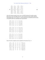
where the subscript outside of each vector on the RHS indicates the member number.
Each of the vectors at the RHS, however, can be expressed in terms of their respective
nodal displacement vector using Eq.12, with the nodal forces and displacements referring
to the global nodal force and displacement representation:
⎪
⎪
⎭
⎪
⎪
⎬
⎫
⎪
⎪
⎩
⎪
⎪
⎨
⎧
2
2
1
1
y

x
y
x
F
F
F
F
=
1
44434241
34333231
24232221
14131211
⎥
⎥
⎥
⎥
⎦
⎤
⎢
⎢
⎢
⎢
⎣
⎡
kkkk
kkkk
kkkk
kkkk
⎪

⎪
⎭
⎪
⎪
⎬
⎫
⎪
⎪
⎩
⎪
⎪
⎨
⎧
2
2
1
1
v
u
v
u
⎪
⎪
⎭
⎪
⎪
⎬
⎫
⎪
⎪

⎩
⎪
⎪
⎨
⎧
3
3
2
2
y
x
y
x
F
F
F
F
=
2
44434241
34333231
24232221
14131211
⎥
⎥
⎥
⎥
⎦
⎤
⎢

⎢
⎢
⎢
⎣
⎡
kkkk
kkkk
kkkk
kkkk
⎪
⎪
⎭
⎪
⎪
⎬
⎫
⎪
⎪
⎩
⎪
⎪
⎨
⎧
3
3
2
2
v
u
v

u
⎪
⎪
⎭
⎪
⎪
⎬
⎫
⎪
⎪
⎩
⎪
⎪
⎨
⎧
3
3
1
1
y
x
y
x
F
F
F
F
=
3
44434241

34333231
24232221
14131211
⎥
⎥
⎥
⎥
⎦
⎤
⎢
⎢
⎢
⎢
⎣
⎡
kkkk
kkkk
kkkk
kkkk
⎪
⎪
⎭
⎪
⎪
⎬
⎫
⎪
⎪
⎩
⎪

⎪
⎨
⎧
3
3
1
1
v
u
v
u
Each of the above equations can be expanded to fit the form of Eq. 14:
1
2
2
1
1
0
0
⎪
⎪
⎪
⎪
⎭
⎪
⎪
⎪
⎪
⎬
⎫

⎪
⎪
⎪
⎪
⎩
⎪
⎪
⎪
⎪
⎨
⎧
y
x
y
x
F
F
F
F
=
1
44434241
34333231
24232221
14131211
000000
000000
00
00
00

00
⎥
⎥
⎥
⎥
⎥
⎥
⎥
⎥
⎦
⎤
⎢
⎢
⎢
⎢
⎢
⎢
⎢
⎢
⎣
⎡
kkkk
kkkk
kkkk
kkkk
⎪
⎪
⎪
⎪
⎭

⎪
⎪
⎪
⎪
⎬
⎫
⎪
⎪
⎪
⎪
⎩
⎪
⎪
⎪
⎪
⎨
⎧
3
3
2
2
1
1
v
u
v
u
v
u
Truss Analysis: Matrix Displacement Method by S. T. Mau

16
2
3
3
2
2
0
0
⎪
⎪
⎪
⎪
⎭
⎪
⎪
⎪
⎪
⎬
⎫
⎪
⎪
⎪
⎪
⎩
⎪
⎪
⎪
⎪
⎨
⎧

y
x
y
x
F
F
F
F
=
2
44434241
34333231
24232221
14131211
00
00
00
00
000000
000000
⎥
⎥
⎥
⎥
⎥
⎥
⎥
⎥
⎦
⎤

⎢
⎢
⎢
⎢
⎢
⎢
⎢
⎢
⎣
⎡
kkkk
kkkk
kkkk
kkkk
⎪
⎪
⎪
⎪
⎭
⎪
⎪
⎪
⎪
⎬
⎫
⎪
⎪
⎪
⎪
⎩

⎪
⎪
⎪
⎪
⎨
⎧
3
3
2
2
1
1
v
u
v
u
v
u
3
3
3
1
1
0
0
⎪
⎪
⎪
⎪
⎭

⎪
⎪
⎪
⎪
⎬
⎫
⎪
⎪
⎪
⎪
⎩
⎪
⎪
⎪
⎪
⎨
⎧
y
x
y
x
F
F
F
F
=
3
44434241
34333231
24232221

14131211
00
00
000000
000000
00
00
⎥
⎥
⎥
⎥
⎥
⎥
⎥
⎥
⎦
⎤
⎢
⎢
⎢
⎢
⎢
⎢
⎢
⎢
⎣
⎡
kkkk
kkkk
kkkk

kkkk
⎪
⎪
⎪
⎪
⎭
⎪
⎪
⎪
⎪
⎬
⎫
⎪
⎪
⎪
⎪
⎩
⎪
⎪
⎪
⎪
⎨
⎧
3
3
2
2
1
1
v

u
v
u
v
u
When each of the RHS vectors in Eq. 14 is replaced by the RHS of the above three
equations, the resulting equation is the unconstrained global stiffness equation:
⎥
⎥
⎥
⎥
⎥
⎥
⎥
⎥
⎦
⎤
⎢
⎢
⎢
⎢
⎢
⎢
⎢
⎢
⎣
⎡
666564636261
565554535251
464544434241

363534333231
262524232221
161514131211
KKKKKK
KKKKKK
KKKKKK
KKKKKK
KKKKKK
KKKKKK
⎪
⎪
⎪
⎪
⎭
⎪
⎪
⎪
⎪
⎬
⎫
⎪
⎪
⎪
⎪
⎩
⎪
⎪
⎪
⎪
⎨

⎧
3
3
2
2
1
1
v
u
v
u
v
u
=
⎪
⎪
⎪
⎪
⎭
⎪
⎪
⎪
⎪
⎬
⎫
⎪
⎪
⎪
⎪
⎩

⎪
⎪
⎪
⎪
⎨
⎧
3
3
2
2
1
1
y
x
y
x
y
x
P
P
P
P
P
P
(15)
where the components of the unconstrained global stiffness matrix, K
ij
, is the
superposition of the corresponding components in each of the three expanded stiffness
matrices in the equations above.

In actual computation, it is not necessary to expand the stiffness equation in Eq. 12 into
the 6-equation form as we did earlier. That was necessary only for the understanding of
how the results are derived. We can use the local-to-global DOF relationship in the
global DOF table and place the member stiffness components directly into the global
stiffness matrix. For example, component (1,3) of the member-2 stiffness matrix is added
to component (3,5) of the global stiffness matrix. This simple way of assembling the
global stiffness matrix is called the Direct Stiffness Method.
To carry out the above procedures numerically, we need to use the dimension and
member property given at the beginning of this section to arrive at the stiffness matrix for
each of the three members:
Truss Analysis: Matrix Displacement Method by S. T. Mau
17
(k
G
)
1
=(
1
22
22
22
22
1
)
⎥
⎥
⎥
⎥
⎥
⎦

⎤
⎢
⎢
⎢
⎢
⎢
⎣
⎡
−−
−−
−−
−−
SCSSCS
CSCCSC
SCSSCS
CSCCSC
L
EA
=
⎥
⎥
⎥
⎥
⎦
⎤
⎢
⎢
⎢
⎢
⎣

⎡
−−
−−
−−
−−
8.126.98.126.9
6.92.76.92.7
8.126.98.126.9
6.92.76.92.7
(k
G
)
2
=(
2
22
22
22
22
2
)
⎥
⎥
⎥
⎥
⎥
⎦
⎤
⎢
⎢

⎢
⎢
⎢
⎣
⎡
−−
−−
−−
−−
SCSSCS
CSCCSC
SCSSCS
CSCCSC
L
EA
=
⎥
⎥
⎥
⎥
⎦
⎤
⎢
⎢
⎢
⎢
⎣
⎡
−−
−−−

−−−
−−
8.126.98.126.9
6.92.76.92.7
8.126.98.126.9
6.92.76.92.7
(k
G
)
3
=(
3
22
22
22
22
3
)
⎥
⎥
⎥
⎥
⎥
⎦
⎤
⎢
⎢
⎢
⎢
⎢

⎣
⎡
−−
−−
−−
−−
SCSSCS
CSCCSC
SCSSCS
CSCCSC
L
EA
=
⎥
⎥
⎥
⎥
⎦
⎤
⎢
⎢
⎢
⎢
⎣
⎡
−
−
06.900
07.1607.16
0000

07.1607.16
When the three member stiffness matrices are assembled according to the Direct Stiffness
Method, the unconstrained global stiffness equation given at the beginning of this section
is obtained. For example, the unconstrained global stiffness matrix component k
34
is the
superposition of (k
34
)
1
of member 1 and (k
12
)
2
of member 2. Note that the unconstrained
global stiffness matrix has the same features as the member stiffness matrix: symmetric
and singular, etc.
5. Constrained Global Stiffness Equation and Its Solution
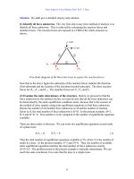
Example 2. Now consider the same three-bar truss as shown before with E=70 GPa,
A=1,430 mm
2
for each member but with the support and loading conditions added.
A constrained and loaded truss in a global coordinate system.
x
y
1
2
4m
3m
2m

2m
3
3m
1
2
3
1.0 MN
0.5 MN
Truss Analysis: Matrix Displacement Method by S. T. Mau
18
Solution. The support conditions are: u
1
=0, v
1
=0, and v
3
=0. The loading conditions are:
P
x2
=0.5 MN, P
y2
= −1.0 MN, and P
x3
=0. The stiffness equation given at the beginning of
the last section now becomes
⎥
⎥
⎥
⎥
⎥

⎥
⎥
⎥
⎦
⎤
⎢
⎢
⎢
⎢
⎢
⎢
⎢
⎢
⎣
⎡
−−
−−
−−−
−−−
−−
−−−
8.126.98.126.900
6.199.236.92.706.16
8.126.96.2508.126.9
6.92.704.146.92.7
008.126.98.126.9
06.166.92.76.99.23
⎪
⎪
⎪

⎪
⎭
⎪
⎪
⎪
⎪
⎬
⎫
⎪
⎪
⎪
⎪
⎩
⎪
⎪
⎪
⎪
⎨
⎧
0
0
0
3
2
2
u
v
u
=
⎪

⎪
⎪
⎪
⎭
⎪
⎪
⎪
⎪
⎬
⎫
⎪
⎪
⎪
⎪
⎩
⎪
⎪
⎪
⎪
⎨
⎧
−
3
1
1
0
0.1
5.0
y
y

x
P
P
P
Note that there are exactly six unknown in the six equations. The solution of the six
unknowns is obtained in two steps. In the first step, we notice that the three equations, 3
rd
through 5
th
, are independent from the other three and can be dealt with separately.
⎥
⎥
⎥
⎦
⎤
⎢
⎢
⎢
⎣
⎡
−
−
9.236.92.7
6.96.250
2.704.14
⎪
⎭
⎪
⎬
⎫

⎪
⎩
⎪
⎨
⎧
3
2
2
u
v
u
=
⎪
⎭
⎪
⎬
⎫
⎪
⎩
⎪
⎨
⎧
−
0
0.1
5.0
(16)
Eq. 16 is the constrained stiffness equation of the loaded truss. The constrained 3x3
stiffness matrix is symmetric but not singular. The solution of Eq. 16 is: u
2

=0.053 m,
v
2
= −0.053 m, and u
3
= 0.037 m. In the second step, the reactions are obtained from the
direct substitution of the displacement values into the other three equations, 1
st
, 2
nd
and
6
th
:
⎥
⎥
⎥
⎦
⎤
⎢
⎢
⎢
⎣
⎡
−−
−−
−−−
8.126.98.126.900
008.126.98.126.9
06.166.92.76.99.23

⎪
⎪
⎪
⎪
⎭
⎪
⎪
⎪
⎪
⎬
⎫
⎪
⎪
⎪
⎪
⎩
⎪
⎪
⎪
⎪
⎨
⎧
−
0
037.0
053.0
053.0
0
0
=

⎪
⎭
⎪
⎬
⎫
⎪
⎩
⎪
⎨
⎧
−
83.0
17.0
5.0
=
⎪
⎭
⎪
⎬
⎫
⎪
⎩
⎪
⎨
⎧
3
1
1
y
y

x
P
P
P
or
⎪
⎭
⎪
⎬
⎫
⎪
⎩
⎪
⎨
⎧
3
1
1
y
y
x
P
P
P
=
⎪
⎭
⎪
⎬
⎫

⎪
⎩
⎪
⎨
⎧
−
83.0
16.0
5.0
MN
The member deformation represented by the member elongation can be computed by the
member deformation equation, Eq. 3:
Truss Analysis: Matrix Displacement Method by S. T. Mau
19
Member 1:
∆
1
=
⎣⎦
1
SCSC −−
⎪
⎪
⎭
⎪
⎪
⎬
⎫
⎪
⎪

⎩
⎪
⎪
⎨
⎧
2
2
1
1
v
u
v
u
=
⎣⎦
1
8.06.08.06.0 −−
⎪
⎪
⎭
⎪
⎪
⎬
⎫
⎪
⎪
⎩
⎪
⎪
⎨

⎧
− 053.0
053.0
0
0
= -0.011m
For member 2 and member 3, the elongations are
∆
2
= −0.052m, and
∆
3
=0.037m.
The member forces are computed using Eq. 1.
F=k
∆
=
L
EA
∆
F
1
= −0.20 MN, F
2
= −1.04 MN, F
3
= 0.62 MN
The results are summarized in the following table.
Nodal and Member Solutions
Displacement (m) Force (MN)

Node
x-direction y-direction x-direction y-direction
1 0 0 -0.50 0.16
2 0.053 -0.053 0.50 -1.00
3 0.037 0 0 0.83
Member Elongation (m) Force (MN)
1 -0.011 -0.20
2 -0.052 -1.04
3 0.037 0.62
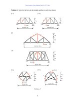
Problem 2. Consider the same three-bar truss as that in Example 2, but with a different
numbering system for members. Construct the constrained stiffness equation, Eq. 16.
Problem 2.
x
y
1
2
4m
3m
2m
2m
3
3m
1
3
2
1.0 MN
0.5 MN
Truss Analysis: Matrix Displacement Method by S. T. Mau
20
6. Procedures of Truss Analysis

Example 3. Consider the following two truss problems, each with member properties
E=70 GPa and A=1,430 mm
2
. The only difference is the existence of an additional
diagonal member in the second truss. It is instructive to see how the analyses and results
differ.
Two truss problems.
Solution. We will carry out a step-by-step solution procedure for the two problems,
referring to the truss at the left and at the right as the first and second truss, respectively.
We also define the global coordinate system in both cases as one with the origin at node 1
and its x-and y-direction coincide with the horizontal and vertical directions, respectively.
(1) Number the nodes and members and define the nodal coordinates.
Nodal Coordinates
Node x (m) y (m)
100
204
334
430
(2) Define member property, starting and end nodes and compute member data.
1 MN
0.5 MN
1
4
3
2
4 m
3 m
1
2
3

4
5
1 MN
0.5 MN
1
4
3
2
4 m
3 m
1
2
3
4
5
6
Truss Analysis: Matrix Displacement Method by S. T. Mau
21
Member Data
Input Data* Computed Data
Member
S Node E Node EA(MN)
∆
x
∆
y L C S EA/L
1 1 2 1000440.01.025.00
2 2 3 1003031.00.033.33
3 3 4 100 0 -4 4 0.0 -1.0 25.00
4 1 4 1003031.00.033.33

5 2 4 100 3 -4 5 0.6 -0.8 20.00
6 1 3 1003450.60.820.00
* S Node and E Node represent Starting and End nodes.
(3) Compute member stiffness matrices.
k
G
=
⎥
⎥
⎥
⎥
⎥
⎦
⎤
⎢
⎢
⎢
⎢
⎢
⎣
⎡
−−
−−
−−
−−
22
22
22
22
SCSSCS

CSCCSC
SCSSCS
CSCCSC
L
EA
Member 1:
(k
G
)
1
=
⎥
⎥
⎥
⎥
⎦
⎤
⎢
⎢
⎢
⎢
⎣
⎡
−
−
250250
0000
250250
0000
Member 2:

(k
G
)
2
=
⎥
⎥
⎥
⎥
⎦
⎤
⎢
⎢
⎢
⎢
⎣
⎡
−
−
0000
033.33033.33
0000
033.33033.33
Member 3:
(k
G
)
3
=
⎥

⎥
⎥
⎥
⎦
⎤
⎢
⎢
⎢
⎢
⎣
⎡
−
−
250250
0000
250250
0000
Member 4:
Truss Analysis: Matrix Displacement Method by S. T. Mau
22
(k
G
)
4
=
⎥
⎥
⎥
⎥
⎦

⎤
⎢
⎢
⎢
⎢
⎣
⎡
−
−
0000
033.33033.33
0000
033.33033.33
Member 5:
(k
G
)
5
=
⎥
⎥
⎥
⎥
⎦
⎤
⎢
⎢
⎢
⎢
⎣

⎡
−−
−−
−−
−−
8.126.9256.9
6.92.76.92.7
256.98.126.9
6.92.76.92.7
Member 6(for the second truss only):
(k
G
)
6
=
⎥
⎥
⎥
⎥
⎦
⎤
⎢
⎢
⎢
⎢
⎣
⎡
−−
−−
−−

−−
8.126.98.126.9
6.92.76.92.7
8.126.98.126.9
6.92.76.92.7
(4) Assemble the unconstrained global stiffness matrix.
In order to use the Direct Stiffness Method to assemble the global stiffness matrix, we
need the following table which gives the global DOF number corresponding to each local
DOF of each member. This table is generated using the member data given in the table in
subsection (2), namely the starting and end nodes data.
Global DOF Number for Each Member
Global DOF Number for MemberLocal DOF
Number
123456*
1 135131
2 246242
3 357775
4 468886
* For the second truss only.
Armed with this table we can easily direct the member stiffness components to the right
location in the global stiffness matrix. For example, the (2,3) component of (k
G
)
5
will be
added to the (4,7) component of the global stiffness matrix. The unconstrained global
stiffness matrix is obtained after all the assembling is done.
For the first truss:
Truss Analysis: Matrix Displacement Method by S. T. Mau
23

K
1
=
⎥
⎥
⎥
⎥
⎥
⎥
⎥
⎥
⎥
⎦
⎤
⎢
⎢
⎢
⎢
⎢
⎢
⎢
⎢
⎢
⎣
⎡
−−−
−−−
−
−
−−−

−−−
−
−
80.3760.900.25080.1260.900
60.953.400060.920.7033.33
00.25000.2500000
00033.33033.3300
8.1260.90080.3760.900.250
60.920.70
33.3360.953.4000
000000.25000.250
033.330000033.33
For the second truss:
K
2
=
⎥
⎥
⎥
⎥
⎥
⎥
⎥
⎥
⎥
⎦
⎤
⎢
⎢
⎢

⎢
⎢
⎢
⎢
⎢
⎢
⎣
⎡
−−−
−−−
−−−
−−−
−−−
−−−
−−−
−−−
80.3760.900.25080.1260.900
60.953.400060.920.7033.33
00.25080.3760.90080.1260.9
0060.952.40033.3360.920.7
8.1260.
90080.3760.900.250
60.920.7033.3360.953.4000
0080.1260.900.25080.3760.9
033.3360.920.70060.953.40
Note that K
2
is obtained by adding (K
G
)

6
to K
1
at the proper locations in columns and
rows 1, 2, 5, and 6 (enclosed in dashed lines above).
(5) Assemble the constrained global stiffness equation.
Once the support and loading conditions are incorporated into the stiffness equations we
obtain:
For the first truss:
⎥
⎥
⎥
⎥
⎥
⎥
⎥
⎥
⎥
⎦
⎤
⎢
⎢
⎢
⎢
⎢
⎢
⎢
⎢
⎢
⎣

⎡
−−−
−−−
−
−
−−−
−−−
−
−
80.3760.900.25080.1260.900
60.953.400060.920.7033.33
00.25000.2500000
00033.33033.3300
8.1260.90080.3760.900.250
60.920.70
33.3360.953.4000
000000.25000.250
033.330000033.33
⎪
⎪
⎪
⎪
⎭
⎪
⎪
⎪
⎪
⎬
⎫
⎪

⎪
⎪
⎪
⎩
⎪
⎪
⎪
⎪
⎨
⎧
0
0
0
4
3
3
2
2
u
v
u
v
u
=
⎪
⎪
⎪
⎪
⎭
⎪

⎪
⎪
⎪
⎬
⎫
⎪
⎪
⎪
⎪
⎩
⎪
⎪
⎪
⎪
⎨
⎧
−
4
0
0
0
0.1
5.0
1
1
y
P
P
P
y

x
For the second truss:
Truss Analysis: Matrix Displacement Method by S. T. Mau
24
⎥
⎥
⎥
⎥
⎥
⎥
⎥
⎥
⎥
⎦
⎤
⎢
⎢
⎢
⎢
⎢
⎢
⎢
⎢
⎢
⎣
⎡
−−−
−−−
−−−
−−−

−−−
−−−
−−−
−−−
80.3760.900.25080.1260.900
60.953.400060.920.7033.33
00.25080.3760.90080.1260.9
0060.952.40033.3360.920.7
8.1260.
90080.3760.900.250
60.920.7033.3360.953.4000
0080.1260.900.25080.3760.9
033.3360.920.70060.953.40
⎪
⎪
⎪
⎪
⎭
⎪
⎪
⎪
⎪
⎬
⎫
⎪
⎪
⎪
⎪
⎩
⎪

⎪
⎪
⎪
⎨
⎧
0
0
0
4
3
3
2
2
u
v
u
v
u
=
⎪
⎪
⎪
⎪
⎭
⎪
⎪
⎪
⎪
⎬
⎫

⎪
⎪
⎪
⎪
⎩
⎪
⎪
⎪
⎪
⎨
⎧
−
4
0
0
0
0.1
5.0
1
1
y
P
P
P
y
x
(6) Solve the constrained global stiffness equation.
The constrained global stiffness equation in either case contains five equations
corresponding to the third through seventh equations (enclosed in dashed lines above)
that are independent from the other three equations and can be solved for the five

unknown nodal displacements.
For the first truss:

⎥
⎥
⎥
⎥
⎥
⎦
⎤
⎢
⎢
⎢
⎢
⎢
⎣
⎡
−
−
−
−−−
53.400060.920.7
000.25000
0033.33033.33
60.90080.3760.9
20.7033.3360.953.40
⎪
⎪
⎪
⎭

⎪
⎪
⎪
⎬
⎫
⎪
⎪
⎪
⎩
⎪
⎪
⎪
⎨
⎧
4
3
3
2
2
u
v
u
v
u
=
⎪
⎪
⎭
⎪
⎪

⎬
⎫
⎪
⎪
⎩
⎪
⎪
⎨
⎧
−
0
0
0
0.1
5.0
For the second truss:

⎥
⎥
⎥
⎥
⎥
⎦
⎤
⎢
⎢
⎢
⎢
⎢
⎣

⎡
−
−
−
−−−
53.400060.920.7
080.3760.900
060.952.40033.33
60.90080.3760.9
20.7033.3360.953.40
⎪
⎪
⎪
⎭
⎪
⎪
⎪
⎬
⎫
⎪
⎪
⎪
⎩
⎪
⎪
⎪
⎨
⎧
4
3

3
2
2
u
v
u
v
u
=
⎪
⎪
⎭
⎪
⎪
⎬
⎫
⎪
⎪
⎩
⎪
⎪
⎨
⎧
−
0
0
0
0.1
5.0
The reactions are computed by direct substitution.

For the first truss:
Truss Analysis: Matrix Displacement Method by S. T. Mau
25

⎥
⎥
⎥
⎦
⎤
⎢
⎢
⎢
⎣
⎡
−−−
−
80.3760.900.25080.1260.900
000000.25000.250
033.330000033.33
⎪
⎪
⎪
⎪
⎭
⎪
⎪
⎪
⎪
⎬
⎫

⎪
⎪
⎪
⎪
⎩
⎪
⎪
⎪
⎪
⎨
⎧
0
0
0
4
3
3
2
2
u
v
u
v
u
=
⎪
⎭
⎪
⎬
⎫

⎪
⎩
⎪
⎨
⎧
4
1
1
y
y
x
P
P
P
For the second truss:

⎥
⎥
⎥
⎦
⎤
⎢
⎢
⎢
⎣
⎡
−−−
−−−
−−−
80.3760.900.25080.1260.900

0080.1260.900.25080.3760.9
033.3360.920.70060.953.40
⎪
⎪
⎪
⎪
⎭
⎪
⎪
⎪
⎪
⎬
⎫
⎪
⎪
⎪
⎪
⎩
⎪
⎪
⎪
⎪
⎨
⎧
0
0
0
4
3
3

2
2
u
v
u
v
u
=
⎪
⎭
⎪
⎬
⎫
⎪
⎩
⎪
⎨
⎧
4
1
1
y
y
x
P
P
P
Results will be summarized at the end of the example.
(7) Compute the member elongations and forces.
For a typical member i:

∆
i
=
⎣⎦
i
SCSC −−
i
v
u
v
u
⎪
⎪
⎭
⎪
⎪
⎬
⎫
⎪
⎪
⎩
⎪
⎪
⎨
⎧
2
2
1
1
F

i
=(k
∆
)
ι
= (
L
EA
∆
)
ι
(8) Summarizing results.
Truss Analysis: Matrix Displacement Method by S. T. Mau
26
Results for the First Truss
Displacement (m) Force (MN)
Node
x-direction y-direction x-direction y-direction
1 0 0 -0.50 0.33
2 0.066 -0.013 0.60 -1.00
3 0.067 0 0 0
4 0.015 0 0 0.67
Member Elongation (m) Force (MN)
1 -0.013 -0.33
20 0
30 0
4 0.015 0.50
5 -0.042 -0.83
Results for the Second Truss
Displacement (m) Force (MN)

Node
x-direction y-direction x-direction y-direction
1 0 0 -0.50 0.33
2 0.033 -0.021 0.60 -1.00
3 0.029 -0.007 0 0
4 0.011 0 0 0.67
Member Elongation (m) Force (MN)
1 -0.021 -0.52
2 -0.004 -0.14
3 -0.008 -0.19
4 0.011 0.36
5 0.030 -0.60
6 0.012 0.23
Note that the reactions at node 1 and 4 are identical in the two cases, but other results are
changed by the addition of one more diagonal member.
(9) Concluding remarks.
If the number of nodes is N and the number of constrained DOF is C, then
(a) the number of simultaneous equations in the unconstrained stiffness equation is
2N.
(b) the number of simultaneous equations for the solution of unknown nodal
displacements is 2N-C.
Truss Analysis: Matrix Displacement Method by S. T. Mau
27
In the present example, both truss problems have five equations for the five unknown
nodal displacements. These equations cannot be easily solved with hand calculation
and should be solved by computer.
Problem 3. The truss shown is made of members with properties E=70 GPa and
A=1,430 mm
2
. Use a computer to find support reactions, member forces, member

elongations, and all nodal displacements for (a) a unit load applied vertically at the
mid-span node of the lower chord members, and (b) a unit load applied vertically at
the first internal lower chord node. Draw the deflected configuration in each case.
Problem 3.
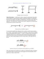
7. Kinematic Stability
In the above analysis, we learned that the unconstrained stiffness matrix is always
singular, because the truss is not yet supported, or constrained. What if the truss is
supported but not sufficiently or properly supported or the truss members are not properly
placed? Consider the following three examples. Each is a variation of the example truss
problem we have just solved.
Three unstable truss configurations
1
4 m
4@3 m = 12 m
Truss Analysis: Matrix Displacement Method by S. T. Mau
28
(1) Truss at left. The three roller supports provide constraints only in the vertical
direction but not in the horizontal direction. As a result, the truss can move in the
horizontal direction indefinitely. There is no resistance to translation in the horizontal
direction.
(2) Truss in the middle. The reactions provided by the supports all point to node 1. As a
result, the reaction forces cannot counter-balance any applied force which produces a
non-zero moment about node 1. The truss is not constrained against rotation about node
1.
(3) Truss at the right. The supports are fine, providing constraints against translation as
well as rotation. The members of the truss are not properly placed. Without a diagonal
member, the truss will change shape as shown. The truss can not maintain its shape
against arbitrarily applied external forces at the nodes.
The first two cases are such that the truss are externally unstable. The last one is
internally unstable. The resistance against changing shape or location as a mechanism is

called kinematic stability. While kinematic stability or instability can be inspected
through visual observation, mathematically it manifests itself in the characteristics of the
constrained global stiffness matrix. If the matrix is singular, then we know the truss is
kinematically unstable. In the example problems in the last section, the two 5x5 stiffness
matrices are both non-singular, otherwise we would not have been able to obtain the
displacement solutions. Thus, kinematic stability of a truss can be tested mathematically
by investigating the singularity of the constrained global stiffness matrix of a truss. In
practice, if the displacement solution appears to be arbitrarily large or disproportionate
among some displacements, then it maybe the sign of an unstable truss configuration.
Sometimes, kinematic instability can be detected by counting constraints or unknown
forces:
External Instability. External Instability happens if there is insufficient number of
constraints. Since it takes at least three constraints to prevent translation and rotation of
an object in a plane, any support condition that provides only one or two constraints will
result in instability. The left truss in the figure below has only two support constraints and
is unstable.
Internal Instability. Internal instability happens if the total number of force unknowns is
less than the number of displacement DOFs. If we denote the number of member force
unknowns as M and support reaction unknowns as R. Then internal instability results if
M+R < 2N. The truss at the right in the figure below has M=4 and R=3 but 2N=8. It is
unstable.
Truss Analysis: Matrix Displacement Method by S. T. Mau
29
Kinematic instability resulting from insufficient number of supports or members.
Problem 4: Discuss the kinematic stability of each of the plane truss shown.
(1) (2)
(3) (4)
(5) (6)
(7) (8)
(9) (10)

Problem 4.
Truss Analysis: Matrix Displacement Method by S. T. Mau
30
8. Summary
The fundamental concept in the displacement method and the procedures of solution are
the following:
(1) If all the key displacement quantities of a given problem are known, then the
deformation of each member can be computed using the conditions of compatibility,
which is manifested in the form of Eq. 2 through Eq. 4.
(2) Knowing the member deformation, we can then compute the member force using the
member stiffness equation, Eq. 1.
(3) The member force of a member can be related to the nodal forces expressed in the
global coordinate system by Eq. 7 or Eq. 8, which is the forced transformation
equation.
(4) The member nodal forces and the externally applied forces are in equilibrium at each
node, as expressed in Eq. 14, which is the global equilibrium equation in terms of
nodal forces.
(5) The global equilibrium equation can then be expressed in terms of nodal
displacements through the use of member stiffness equation, Eq. 11. The result is the
global stiffness equation in terms of nodal displacements, Eq. 15.
(6) Since not all the nodal displacements are known, we can solve for the unknown
displacements from the constrained global stiffness equation, Eq. 16 in Example 3.
(7) Once all the nodal forces are computed, the remaining unknown quantities are
computed by simple substitution.
The displacement method is particularly suited for computer solution because the
solution steps can be easily programmed through the direct stiffness method of
assembling the stiffness equation. The correct solution can always be computed if the
structure is stable ( kinematically stable), which means the structure is internally properly
connected and externally properly supported to prevent it from becoming a mechanism
under any loading conditions.

31
Truss Analysis: Force Method, Part I
1. Introduction
In the chapter on matrix displacement method of truss analysis, truss analysis is
formulated with nodal displacement unknowns as the fundamental variables to be
determined. The resulting method of analysis is simple and straightforward and is very
easy to be implemented into a computer program. As a matter of fact, virtually all
structural analysis computer packages are coded with the matrix displacement method.
The one drawback of the matrix displacement method is that it does not provide any
insight on how the externally applied loads are transmitted and taken up by the members
of the truss. Such an insight is critical when an engineer is required not only to analyze a
given truss but also to design a truss from scratch.
We will now introduce a different approach, the force method. The essence of the force
method is the formulation of the governing equations with the forces as unknown
variables. The beginning point of the force method is the equilibrium equations
expressed in terms of forces. Depending on how the free-body-diagrams are selected to
develop these equilibrium equations, we may use either the method of joint or the method
of section or a combination of both to solve a truss problem.
In the force method of analysis, if the force unknowns can be solved by the equilibrium
equations alone, then the solution process is very straightforward: finding member forces
from equilibrium equations, finding member elongation from member forces, and finding
nodal displacements from member elongation. Assuming that the trusses considered
herein are all kinematically stable, the only other pre-requisite for such a solution
procedure is that the truss be a statically determinate one, i.e., the total number of force
unknowns is equal to the number of independent equilibrium equations. In contrast, a
statically indeterminate truss, which has more force unknowns than the number of
independent equilibrium equations, requires the introduction of additional equations
based on the geometric compatibility or consistent deformations to supplement the
equilibrium equations. We shall study the statically determinate problems first,
beginning by a brief discussion of determinacy and truss types.

2. Statically Determinate Plane Truss Types
For statically determinate trusses, the force unknowns, consisting of M member forces if
there are M members, and R reactions, are equal in number to the equilibrium equations.
Since one can generate two equilibrium equations from each node, the number of
independent equilibrium equations is 2N, where N is the number of nodes. Thus by
definition M+R=2N is the condition of statical determinacy. This is to assume that the
truss is stable, because it is meaningless to ask whether the truss is determinate if it is not
stable. For this reason, stability of a truss should be examined first. One class of plane
Truss Analysis: Force Method, Part I by S. T. Mau
32
trusses, called simple truss, is always stable and determinate if properly supported
externally. A simple truss is a truss built from a basic triangle of three bars and three
nodes by adding two-bar-and-a-node one at a time. Examples of simple trusses are shown
below.
Simple trusses.
The basic triangle of three bars (M=3) and three nodes (N=3) is a stable configuration and
satisfies M+R=2N if there are three reaction forces (R=3). Adding two bars and a node
creates a different but stable configuration. The two more force unknowns from the two
bars are compensated exactly by the two equilibrium equations from the new node. Thus,
M+R=2N is still satisfied.
Another class of plane truss is called compound truss. A compound truss is a truss
composed of two or more simple trusses linked together. If the linkage consists of three
bars placed properly, not forming parallel or concurrent forces, then a compound truss is
also stable and determinate. Examples of stable and determinate compound trusses are
shown below, where the dotted lines cut across the links.
Compound trusses.
Truss Analysis: Force Method, Part I by S. T. Mau
33
A plane truss can neither be classified as a simple truss nor a compound truss is called a
complex truss. A complex truss is best solved by the computer version of the method of

joint to be described later. A special method, called method of substitution, was
developed for complex trusses in the pre-computer era. It has no practical purposes
nowadays and will not be described herein. Two complex trusses are shown below, the
one at left is stable and determinate and the other at right is unstable. The instability of
complex trusses cannot be easily determined. There is a way, however: self-equilibrium
test. If we can find a system of internal forces that are in equilibrium by themselves
without any externally applied loads, then the truss is unstable. It can be seen that the
truss at right can have the same tension force of any magnitude, S, in the three internal
bars and compression force, -S, in all the peripheral bars, and they will be in equilibrium
without any externally applied forces.
Stable and unstable complex trusses.
Mathematically such a situation indicates that there will be no unique solution for any
given set of loads, because the self-equilibrium “solution” can always be superposed onto
any set of solution and creates a new set of solution. Without a unique set of solution is a
sign that the structure is unstable.
We may summarize the above discussions with the following conclusions:
(1) Stability can often determined by examining the adequacy of external supports and
internal member connections. If M+R<2N, however, then it is always unstable,
because there is not enough number of members or supports to provide adequate
constraints to prevent a truss from turning into a mechanism under certain loads.
(2) For a stable plane truss, if M+R=2N, then it is statically determinate.
(3) A simple truss is stable and determinate.
(4) For a stable plane truss, if M+R>2N, then it is statically indeterminate. The
discrepancy between the two numbers, M+R–2N, is called the degrees of
indeterminacy, or the number of redundant forces. Statically indeterminate truss
problems cannot be solved by equilibrium conditions alone. The conditions of
compatibility must be utilized to supplement the equilibrium conditions. This way of
solution is called method of consistent deformations and will be described in Part II.
Examples of indeterminate trusses are shown below.
60

o
60
o
60
o
60
o
60
o
60
o
Truss Analysis: Force Method, Part I by S. T. Mau
34
Statically indeterminate trusses.
The truss at the left is statically indeterminate to the first degree because there are one
redundant reaction force: M=5, R=4, and M+R-2N=1. The truss in the middle is also
statically indeterminate to the first degree because of one redundant member: M=6, R=3,
and M+R-2N=1. The truss at the right is statically indeterminate to the second degree
because M=6, R=4 and M+R-2N=2.
3. Method of Joint and Method of Section
The method of joint draws its name from the way a FBD is selected: at the joints of a
truss. The key to the method of joint is the equilibrium of each joint. From each FBD,
two equilibrium equations are derived. The method of joint provides insight on how the
external forces are balanced by the member forces at each joint, while the method of
section provides insight on how the member forces resist external forces at each
“section”. The key to the method of section is the equilibrium of a portion of a truss
defined by a FBD which is a portion of the structure created by cutting through one or
more sections. The equilibrium equations are written from the FBD of that portion of the
truss. There are three equilibrium equations as oppose to the two for a joint.
Consequently, we make sure there are no more than three unknown member forces in the

FBD when we choose to cut through a section of a truss. In the following example
problems and elsewhere, we use the terms “joint” and “node” as interchangeable.
Example 1. Find all support reactions and member forces of the loaded truss shown.
A truss problem to be solved by the method of joint.
x
y
1
2
4m
3m
3
3m
1
2
3
1.0 kN
0.5 kN
1
4
1
3
4
5
1
4
32
1
2
3
4

5
2
1
4
32
1
3
4
5
6