Fundamentals of Structural Analysis Episode 1 Part 4 pptx

Truss Analysis: Force Method, Part I by S. T. Mau
55
Problem 2. Solve for the force in the marked members in each truss shown.
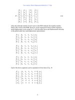
(1-a)(1-b)
(2)
(3)
(4-a)(4-b)
Problem 2.
4m
4@3m=12m
1 kN
a
b
4m
4@3m=12m
1 kN
a
b
12 kN
4 @ 4m=16 m
2m
3m
a
b
c
6@3m=18m
4m
4m
12 kN
a
b

c
3@3m=9m
4m
4m
15 kN
a
AB
b
c
3@3m=9m
4m
4m
15 kN
a
AB
b
Truss Analysis: Force Method, Part I by S. T. Mau
56
4. Matrix Method of Joint
The development of the method of joint and the method of section pre-dates the advent of
electronic computer. Although both methods are easy to apply, it is not practical for
trusses with many members or nodes especially when all member forces are needed. It
is, however, easy to develop a matrix formulation of the method of joint. Instead of
manually establishing all the equilibrium equations from each joint or from the whole
structure and then put the resulting equations in a matrix form, there is an automated way
of assembling the equilibrium equations as shown herein.
Assuming there are N nodes and M member force unknowns and R reaction force
unknowns and 2N=M+R for a given truss, we know there will be 2N equilibrium
equations, two from each joint. We shall number the joints or nodes from one to N. At
each joint, there are two equilibrium equations. We shall define a global x-y coordinate

system that is common to all joints. We note, however, it is not necessary for every node
to have the same coordinate system, but it is convenient to do so. The first equilibrium
equation at a node will be the equilibrium of forces in the x-direction and the second will
be for the y-direction. These equations are numbered from one to 2N in such a way that
the x-direction equilibrium equation from the ith node will be the (2i-1)th equation and
the y-direction equilibrium equation from the same node will be the (2i)th equation. In
each equation, there will be terms coming from the contribution of member forces,
externally applied forces, or reaction forces. We shall discuss each of these forces and
develop an automated way of establishing the terms in each equilibrium equation.
Contribution from member forces. A typical member, k, having a starting node, i, and
an ending node, j, is oriented with an angle
θ
from the x-axis as shown.
Member orientation and the member force acting on member-end and nodes.
The member force, assumed to be tensile, pointing away from the member at both ends
and in opposite direction when acting on the nodes, contributes to four nodal equilibrium
equations at the two end nodes (we designate the RHS of an equilibrium equation as
positive and put the internal nodal forces to the LHS):
(2i-1)th equation (x-direction): (−Cos
θ
)F
k
to the LHS
(2i)th equation (y-direction): (−Sin
θ
)F
k
to the LHS
(2j-1)th equation (x-direction): (Cos
θ

)F
k
to the LHS
k
i
j
x
y
θ
k
i
j
θ
F
k
F
k
θ
F
k
F
k
θ
i
j
Truss Analysis: Force Method, Part I by S. T. Mau
57
(2j)th equation (y-direction): (Sin
θ
)F

k
to the LHS
Contribution from externally applied forces. An externally applied force, applying at
node i with a magnitude of P
n
making an angle
α
from the x-axis as shown, contributes
to:
Externally applied force acting at a node.
(2i-1)th equation (x-direction): (Cos
α
)P
n
to the RHS
(2i)th equation (y-direction): (Sin
α
)P
n
to the RHS
Contribution from reaction forces. A reaction force at node i with a magnitude of R
n
making an angle
β
from the x-axis as shown, contributes to:
Reaction force acting at a node.
(2i-1)th equation (x-direction): (-Cos
β
)R
n

to the LHS
(2i)th equation (y-direction): (-Sin
β
)R
n
to the LHS
Input and solution procedures. From the above definition of forces, we can develop
the following solution procedures.
(1) Designate member number, global node number, global nodal coordinates, and
member starting and end node numbers. From these input, we can compute member
length, l, and other data for each member with starting node i and end node j:
∆
x = x
j
−x
i
;
∆
y = y
j
−y
i
; L=
22
)()( yx
∆∆
+
; Cos
θ
=

L
x
∆
; Sin
θ
=
L
y
∆
.
(2) Define reaction forces, including where the reaction is at and the orientation of the
reaction, one at a time. The cosine and sine of the orientation of the reaction force
should be input directly.
(3) Define externally applied forces, including where the force is applied and the
magnitude and orientation, defined by the cosine and sine of the orientation angle.
i
α
i
β
R
n
P
n
Truss Analysis: Force Method, Part I by S. T. Mau
58
(4) Compute the contribution of member forces, reaction forces, and externally applied
forces to the equilibrium equation and place them to the matrix equation. The force
unknowns are sequenced with the member forces first, F
1
, F

2
,…F
M
, followed by
reaction force unknowns, F
M+1
, F
M+2
,…,F
M+R
.
(5) Use a linear simultaneous algebraic equation solver to solve for the unknown forces.
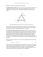
Example 11. Find all support reactions and member forces of the loaded truss shown.
A truss problem to be solved by the matrix method of joint.
Solution. We shall provide a step-by-step solution.
(1) Designate member number, global node number, global nodal coordinates, and
member starting and end node numbers and compute member length, L, and other
data for each member.
Nodal Input Data
Node x-coordinate y-coordinate
1 0.0 0.0
2 3.0 4.0
3 6.0 0.0
Member Input and Computed Data
Member
Start
Node
End
Node
∆

x
∆
y L Cos
θ
Sin
θ
1 1 2 3.0 4.0 5.0 0.6 0.8
2 2 3 3.0 -4.0 5.0 0.6 -0.8
3 1 3 6.0 0.0 6.0 1.0 0.0
(2) Define reaction forces.
x
y
1
2
4m
3m
3
3m
1
2
3
1.0 kN
0.5 kN
Truss Analysis: Force Method, Part I by S. T. Mau
59
Reaction Force Data
Reaction At Node
Cos
β
Sin

β
1 1 1.0 0.0
2 1 0.0 1.0
3 3 0.0 1.0
(3) Define externally applied forces.
Externally Applied Force Data
Force At Node Magnitude
Cos
α
Sin
α
1 2 0.5 1.0 0.0
2 2 1.0 0.0 -1.0
(4) Compute the contribution of member forces, reaction forces, and externally applied
forces to the equilibrium equations and set up the matrix equation.
Contribution of Member Forces
Equation Number and Value of Entry
Member
Number
Force
Number
2i-1 Coeff. 2i Coeff. 2j-1 Coeff. 2j Coeff.
111
−0.6
2
−0.8
3 0.6 4 0.8
223
−0.6
4 0.8 5 0.6 6

−0.8
331
−1.0
2 0.0 5 1.0 6
−0.0
Contribution of Reaction Forces
Equation Number and Value of EntryReaction
Number
Force
Number
2i-1 Coeff. 2i Coeff.
1 4 1 -1.0 2 0.0
2 5 1 0.0 2 -1.0
3 6 5 0.0 6 -1.0
Contribution of Externally Applied Forces
Equation Number and Value of EntryApplied
Force
2i-1 Coeff. 2i Coeff.
1 1 1.0 2 0.0
2 1 0.0 2 1.0
3 5 0.0 6 1.0
Using the above data, we obtain the equilibrium equation in matrix form:
Truss Analysis: Force Method, Part I by S. T. Mau
60
⎥
⎥
⎥
⎥
⎥
⎥

⎥
⎥
⎥
⎥
⎦
⎤
⎢
⎢
⎢
⎢
⎢
⎢
⎢
⎢
⎢
⎢
⎣
⎡
−−
−
−−
−−−
0.1000.08.00
0.0000.16.00
00008.08.0
00006.06.0
00.10.00.008.0
00.00.10.106.0
⎪
⎪

⎪
⎪
⎪
⎭
⎪
⎪
⎪
⎪
⎪
⎬
⎫
⎪
⎪
⎪
⎪
⎪
⎩
⎪
⎪
⎪
⎪
⎪
⎨
⎧
6
5
4
3
2
1

F
F
F
F
F
F
=
⎪
⎪
⎪
⎪
⎪
⎭
⎪
⎪
⎪
⎪
⎪
⎬
⎫
⎪
⎪
⎪
⎪
⎪
⎩
⎪
⎪
⎪
⎪

⎪
⎨
⎧
−
0
0
0.1
5.0
0
0
(5) Solve for the unknown forces. An equation solver produces the following solutions,
where the units are added by the user:
F
1
= −0.21 kN; F
2
= −1.04 kN; F
3
= 0.62 kN;
F
4
= −0.50 kN; F
5
= 0.17 kN; F
6
= 0.83 kN;
Truss Analysis: Force Method, Part I by S. T. Mau
61
Problem 3.
(1) The loaded truss shown is different from that in Example 11 only in the externally

applied loads. Modify the results of Example 11 to establish the matrix equilibrium
equation for this problem.
Problem 3-1.
(2) Establish the matrix equilibrium equation for the loaded truss shown.
Problem 3-2.
x
y
1
2
4m
3m
3
3m
1
2
3
1.0 kN
0.5 kN
x
y
1
2
4m
3m
3
3m
1
2
1.0 kN
0.5 kN

Truss Analysis: Force Method, Part I by S. T. Mau
62
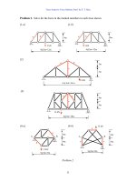
Force transfer matrix. Consider the same three-bar truss as in the previous example
problems. If we apply a unit force one at a time at one of the six possible positions, i.e. x-
and y-directions at each of the three nodes, we have six separate problems as shown
below.
Truss with unit loads.
The matrix equilibrium equation for the first problem appears in the following form:
x
y
1
2
4m
3m
3
3m
1
2
3
x
y
1
2
4m
3m
3
3m
1
2
3

x
y
1
2
4m
3m
3
3m
1
2
3
x
y
1
2
4m
3m
3
3m
1
2
3
x
y
1
2
4m
3m
3
3m

1
2
3
x
y
1
2
4m
3m
3
3m
1
2
3
1 kN
1 kN
1 kN
1 kN
1 kN
1 kN
Truss Analysis: Force Method, Part I by S. T. Mau
63
⎥
⎥
⎥
⎥
⎥
⎥
⎥
⎥

⎥
⎥
⎦
⎤
⎢
⎢
⎢
⎢
⎢
⎢
⎢
⎢
⎢
⎢
⎣
⎡
−−
−
−−
−−−
0.1000.08.00
0.0000.16.00
00008.08.0
00006.06.0
00.10.00.008.0
00.00.10.106.0
⎪
⎪
⎪
⎪

⎪
⎭
⎪
⎪
⎪
⎪
⎪
⎬
⎫
⎪
⎪
⎪
⎪
⎪
⎩
⎪
⎪
⎪
⎪
⎪
⎨
⎧
6
5
4
3
2
1
F
F

F
F
F
F
=
⎪
⎪
⎪
⎪
⎪
⎭
⎪
⎪
⎪
⎪
⎪
⎬
⎫
⎪
⎪
⎪
⎪
⎪
⎩
⎪
⎪
⎪
⎪
⎪
⎨

⎧
0
0
0
0
0
1
(2)
The RHS of the equation is a unit vector. For the other five problems the same matrix
equation will be obtained only with the RHS changed to unit vectors with the unit load at
different locations. If we compile the six RHS vectors into a matrix, it becomes an
identity matrix:
⎥
⎥
⎥
⎥
⎥
⎥
⎥
⎥
⎥
⎥
⎦
⎤
⎢
⎢
⎢
⎢
⎢
⎢

⎢
⎢
⎢
⎢
⎣
⎡
100000
010000
001000
000100
000010
000001
= I (3)
The six matrix equations for the six problems can be put into a single matrix equation, if
we define the six-by-six matrix at the LHS of Eq. 2 as matrix A,
⎥
⎥
⎥
⎥
⎥
⎥
⎥
⎥
⎥
⎥
⎦
⎤
⎢
⎢
⎢

⎢
⎢
⎢
⎢
⎢
⎢
⎢
⎣
⎡
−−
−
−−
−−−
0.1000.08.00
0.0000.16.00
00008.08.0
00006.06.0
00.10.00.008.0
00.00.10.106.0
= A (4)
and the six force unknown vectors as a single six-by-six matrix F:
A
6x6
F
6x6
= I
6x6
(5)
Truss Analysis: Force Method, Part I by S. T. Mau
64

The solution to the six problems, obtained by solving the six problems one at a time, can
be compiled into the single matrix F:
F
6x6
=
⎥
⎥
⎥
⎥
⎥
⎥
⎥
⎥
⎥
⎥
⎦
⎤
⎢
⎢
⎢
⎢
⎢
⎢
⎢
⎢
⎢
⎢
⎣
⎡
−−

−−−
−−−
−
−
0.10.05.067.00.00.0
0.00.05.067.00.10.0
0.00.10.00.10.00.1
0.00.138.05.00.00.0
0.00.063.083.
00.00.0
0.00.063.083.00.00.0
(6)
where each column of the matrix F is a solution to a unit load problem. Matrix F is
called the force transfer matrix. It transfers a unit load into the member force and
reaction force unknowns. It is also the “inverse” of the matrix A, as apparent from Eq. 5.
We can conclude: The nodal equilibrium conditions are completely characterized by the
matrix A, the inverse of it, matrix F , is the force transfer matrix, which transfers any unit
load into member and reaction forces.
If the force transfer matrix is known, either by solving the unit load problems one at a
time or by solving the matrix equation, Eq. 5, with an equation solver, then the solution to
any other loads can be obtained by a linear combination of the force transfer matrix.
Thus the force transfer matrix also characterizes completely the nodal equilibrium
conditions of the truss. The force transfer matrix is particularly useful if there are many
different loading conditions that one wants to solve for. Instead of solving for each loads
separately, one can solve for the force transfer matrix, then solve for any other load by a
linear combination as shown in the following example.
Example 12. Find all support reactions and member forces of the loaded truss shown,
knowing that the force transfer matrix is given by Eq. 6.
A truss problem to be solved with the force transfer matrix.
x

y
1
2
4m
3m
3
3m
1
2
3
1.0 kN
0.5 kN
Truss Analysis: Force Method, Part I by S. T. Mau
65
Solution. The given loads can be cast into a load vector, which can be easily computed as
the combination of the third and fourth unit load vectors as shown below.
⎪
⎪
⎪
⎪
⎪
⎭
⎪
⎪
⎪
⎪
⎪
⎬
⎫
⎪

⎪
⎪
⎪
⎪
⎩
⎪
⎪
⎪
⎪
⎪
⎨
⎧
−
0
0
0.1
5.0
0
0
= (0.5)
⎪
⎪
⎪
⎪
⎪
⎭
⎪
⎪
⎪
⎪

⎪
⎬
⎫
⎪
⎪
⎪
⎪
⎪
⎩
⎪
⎪
⎪
⎪
⎪
⎨
⎧
0
0
0
0.1
0
0
+ (−1.0)
⎪
⎪
⎪
⎪
⎪
⎭
⎪

⎪
⎪
⎪
⎪
⎬
⎫
⎪
⎪
⎪
⎪
⎪
⎩
⎪
⎪
⎪
⎪
⎪
⎨
⎧
0
0
0.1
0
0
0
(7)
The solution is then the same linear combination of the third and fourth vectors of the
force transfer matrix:
⎪
⎪

⎪
⎪
⎪
⎭
⎪
⎪
⎪
⎪
⎪
⎬
⎫
⎪
⎪
⎪
⎪
⎪
⎩
⎪
⎪
⎪
⎪
⎪
⎨
⎧
6
5
4
3
2
1

F
F
F
F
F
F
= (0.5)
⎪
⎪
⎪
⎪
⎪
⎭
⎪
⎪
⎪
⎪
⎪
⎬
⎫
⎪
⎪
⎪
⎪
⎪
⎩
⎪
⎪
⎪
⎪

⎪
⎨
⎧
−
−
−
67.0
67.0
0.1
5.0
83.0
83.0
+ (−1.0)
⎪
⎪
⎪
⎪
⎪
⎭
⎪
⎪
⎪
⎪
⎪
⎬
⎫
⎪
⎪
⎪
⎪

⎪
⎩
⎪
⎪
⎪
⎪
⎪
⎨
⎧
−
−
−
5.0
5.0
0.0
38.0
63.0
63.0
=
⎪
⎪
⎪
⎪
⎪
⎭
⎪
⎪
⎪
⎪
⎪

⎬
⎫
⎪
⎪
⎪
⎪
⎪
⎩
⎪
⎪
⎪
⎪
⎪
⎨
⎧
−
−
−
83.0
17.0
50.0
62.0
04.1
21.0
kN
Truss Analysis: Force Method, Part I by S. T. Mau
66
Problem 4.
(1) The loaded truss shown is different from that in Example 11 only in the externally
applied loads. Use the force transfer matrix of Eq. 6 to find the solution.

Problem 4-1.
(2) The loaded truss shown is different from that in Example 11 only in the externally
applied loads. Use the force transfer matrix of Eq. 6 to find the solution.
Problem 4-2.
x
y
1
2
4m
3m
3
3m
1
2
3
1.0 kN
0.5 kN
x
y
1
2
4m
3m
3
3m
1
2
3
1.0 kN
0.5 kN

1.0 kN
67
Truss Analysis: Force Method, Part II
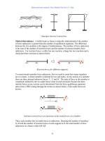
5.Truss Deflection
A truss has a designed geometry and an as-built geometry. Displacement of nodes from
their designed positions can be caused by manufacuring or construction errors.
Displacement of nodes from their as-built positions is induced by applied loads or
temperature changes. Truss deflection refers to either deviastion from the designed
postions or from the as-built positions. No matter what is the cause for deflection, one or
more members of the truss may have experienced a change of length. Such a change of
length makes it necessary for the truss to adjust to the change by displacing the nodes
from its original position as shown below. Truss deflection is the result of displacements
of some or all of the truss nodes and nodal displacements are caused by the change of
length of one or more members.
Elongation of member 3 induces nodal displacements and truss deflection.
From the above figure, it is clear that geometric relations determine nodal displacements.
In fact, nodal displacements can be obtained graphically for any given length changes as
illustrated below.
Displacements of nodals 3 and 2 determined graphically.
Even for more complex truss geometry than the above, a graphyical method can be
developed to determine all the nodal displacements. In the age of computers, however,
such a graphical method is no longer practical and necessary. Truss nodal displacements
can be computed using the matrix displacment method or, as we shall see, using the force
1
2
3
1
2
3
3

1
2
3
1
2
3
3
2
Truss Analysis: Force Method, Part II by S.T.Mau
68
method, especially when all the membe elongations are known. The method we shall
introduce is the unit-load method, the derivation of which requires an understanding of
the concept of work done by a force. A brief review of the concept follows.
Work and Virtual Work. Consider a bar fixed at one end and being pulled at the other
end by a force P. The displacement at the point of application of the force P is
∆
as
shown in the figure below.
Force and displacement at the point of application of the force.
As assumed throughout the text, the force is considered a static force, i.e., its application
is such that no dynamic effects are induced. To put it simply, the force is applied
graudally, starting from zero and increasing its magnitude slowly until the final
magnitude P is reached. Consequently, as the force is applied, the displacement increases
from zero to the final magnitude
∆
proportionally as shown below, assuming the material
is linearly elastic.
Force-displacement relationship.
The work done by the force P is the integration of the force-displacement function and is
equal to the triangular area shown above. Denoting work by W we obtain

W=
2
1
P
∆
(8)
Now, consider two additional cases of load-displacement after the load P is applied: The
first is the case with the load level P held constant and an additional amount of
displacement
δ
is induced. If the displacement is not real but one which we imagined as
happening, then the displacement is called a virtual displacement. The second is the case
with the displacement level held constant, but an additional load p is applied. If the load
is not real but one which we imagined as happening, then the force is called a virtual
∆
P
∆
P
D
isplacement
F
orce
Truss Analysis: Force Method, Part II by S.T.Mau
69
force. In both cases, we can construct the load-displacement history as shown in the
figures below.
A case of virtual displacement (left) and a case of virtual force (right).
The additional work done is called virtual work in both cases, although they are induced
with different means. The symbol for virtual work is
δ

W, which is to be differentiated
from dW, the real increment of W. The symbol
δ
can be considered as an operator that
generates an virtual increment just as the symbol d is an operator that generates an actual
increment. From the above figures, we can see that the virual work is different from the
real work in Eq. 8.
δ
W= P
δ
due to virtual displacement
δ
.(9)
δ
W= p
∆
due to virtual force p. (10)
In both cases, the factor _ in Eq. 8 are not present.
Energy Principles. The work or virtual work by itself does not provide any equations for
the anaylsis of a structure, but they are associated with numerous energy principles that
contain useful equations for structureal analysis. We will introduce only three.
(1) Conservation of Mechanical Enengy. This principle states that the work done by all
external forces on a system is equal to the work done by all internal forces in the system
for a system in equilibrium.
W
ext
=W
int
(11)
where

W
ext
= work done by external forces, and
W
int
= work done by internal forces.
∆
P
D
isp.
F
orce
∆
D
isp.
F
orce
P
δ
p
Truss Analysis: Force Method, Part II by S.T.Mau
70
Example 13. Find the displacement at the loaded end, given the bar shown has a
Young’s modulus E, cross-sectional area A, and length L.
Example problem on conservation of mechanical energy.
Solution. We can use Eq. 11 to find the tip displacement
∆
. The internal work done can
be computed using the information contained in the following figure.
Internal forces acting on an infinitesimal element.

The elongation of the infinitesimal element, d
∆
, is related to the axial force P by
d
∆
=
ε
dx =
E
dx
σ
=
EA
Pdx
where
ε
and
σ
are the nromal strain and stress in the axial direction, respectively. The
interal work done by P on the infinitesimal element is then
dW
int
=
2
1
P(d
∆
) =
2
1

P(
EA
Pdx
)
The total internal work done is the sum of the work over all the infinitesimal elements:
W
int
= ∫ dW = ∫
2
1
P(
EA
Pdx
) =
2
1
EA
LP
2
The external work done is simply:
W
ext
=
2
1
P
∆
Eq. 11 leads to
∆
P

∆
P
P
P
x
dx
d
∆
Truss Analysis: Force Method, Part II by S.T.Mau
71
2
1
P
∆
=
2
1
EA
LP
2
From which, we obtain
∆
=
EA
PL
This is of course the familiar formula for the elongation of an axially loaded prismatic
bar. We went through the derivation to show how the principle of conservation of energy
is applied. We note the limitations of the energy conservation principle: unless there is a
single applied load and the dispalcement we want is the displacement at the point of
application of the single load, the energy conservation equation, Eq. 11, is not very useful

for finding displacements. This energy conservation principle is often used for the
derivation of other useful formulas.
(2) Principle of Virtual Displacement. Imagin a virtual displacement or displacement
system is imposed on a structure after a real load syetem has already been applied to the
structure. This principle is expressed as
δ
W =
δ
U (12)
where
δ
W = virtual work done by external forces upon the virtual displacement.
δ
U = virtual work done by internal forces upon the virtual displacement.
The application of Eq. 12 will produce an equlibrium equation relating the external forces
to the internal forces. This principle is sometimes referred to as the Principle of Virtual
Work. It is often used in conjunction with the displacement method of analysis. Since
we are developing the force method of analysis herein, we shall not explore the
application of this principle further at this point.
(3) Principle of Virtual Force − Unit Load Method. In equation this principle is
expressed as

δ
W =
δ
U (13)
where
δ
W = work done by external virtual force(s) upon a real displacement system.
δ

U = work done by internal virtual forces upon a real displacement system.
We illustrate this principle in the context of the truss problems. Consider a truss system
represented by rectangular boxes in the figures below.
Truss Analysis: Force Method, Part II by S.T.Mau
72
A real system (left) and a virtual load system (right).
The left figure represents a truss with known member elongations, V
j
, j =1, 2,…M. The
cause of the elongation is not relevant to the principle of virtual force. We want to find
the displacement,
∆
o
, in certain direction at a point “o”. We create an identical truss and
apply an imaginary (virtual) unit load at point “o” in the direction we want as shown in
the right figure. The unit load produces a system of internal member forces f
j
, j =1,
2,…M.
The work done by the unit load (virutal system) upon the real displacement is
δ
W = 1 (
∆
o
)
The work done by internal virtual forces upon a real displacement system (elongation of
each member) is
δ
U =
j

M
j
j
Vf
∑
=1
The principle of virtual force states that
1 (
∆
o
) =
j
M
j
j
Vf
∑
=1
(14)
Eq. 14 gives the displacement we want. It also shows how simply one can compute the
displacement. Only two sets of data are needed: the elongation of each member and the
internal virtual force of each member corresponding to the virtual unit load.
Before we give a proof of the principle, we shall illustrate the application of it in the
following example.
Example 14. Find the vertical displacement at node 2 of the truss shown, given (a) bar 3
has experienced a temperature increase of 14
o
C, (b) bar 3 has a manufacturing error of 1
mm. overlength, and (c) a horizontal load of 16 kN has been applied at node 3 acting
Member Elongation

V
j
, j =1, 2,…M
Virtual Member Force
f
j
, j =1, 2,…M
∆
o
1
o
o
Truss Analysis: Force Method, Part II by S.T.Mau
73
toward right. All bars have Young’s modulus E= 200 GPa, cross-sectional area A=500
mm
2
, and length L as shown. The linear thermal expansion coefficient is
α
=1.2(10
-5
)/
o
C.
Example for the unit load method.
Solution. All three conditions result in the same consequences, the elongation of member
3 only, but nodes 2 and 3 will be displaced as a result. Denoting the elongation of
memebr 3 as V
3
. We have

(a) V
3
=
α
(
∆
T)L= 1.2(10
-5
)/
o
C (14
o
C) (6,000 mm)= 1mm.
(b) V
3
=1mm.
(c) V
3
= 16 kN (6 m)/[200(10
6
) kN/m
2
(500)(10
-6
)m
2
]=0.001 m= 1mm.
Next we need to find f
3
. Note that we do not need f

1
and f
2
because V
1
and V
2
are both
zero. Still we need to solve the unit-load problem posed in the following figure in order
to find f
3
.
A vitual load system with an applied unit load.
The member forces are easily obtained and f
3
=0.375 kN for the given downward unit
load. A direct application of Eq. 14 yields
1 kN (
∆
o
) =
j
M
j
j
Vf
∑
=1
= f
3

V
3
= 0.375 kN (1 mm)
and
1
2
4m
3m
3
3m
12
3
1
2
4m
3m
3
3m
12
3
1 kN
Truss Analysis: Force Method, Part II by S.T.Mau
74
∆
o
= 0.38 mm. (downward)
We now give a derivation of this principle in the context of truss member elongation
caused by applied loads. Consider a truss system, represented by the rectangular boxes in
the figures below, loaded by two different loading systems – a real load system and a
virtual unit load. The real load system is the actual load applied to the truss under

consideration. The unit load is a virtual load of unit magnitude applied at a point whose
displacement we want and applied in the direction of the displacment we want. These
loads are shown outside of the boxes together with the displacements under the loads.
The corresponding internal member force and member elogation are shown inside of the
boxes.
A real system (left) and a virtual system (right).
In the above figure,
P
i
: the ith applied real load,
∆
i
: the real displacement under the ith applied load,
∆
o
: the displacement we want to find,
F
j
: the ith member force due to the applied real load,
V
j
: the ith member elongation due to the applied real load,
f
j
: the jth member force due to the virtual unit load,
v
j
: the jth member elongation due to the virtual unit load,
∆
i

'
: the displacements in the direction of the ith real applied load but induced by
the virtual unit load.
We will now consider three loading cases:
(1) The case of externally applied loads act alone. The applied loads, P
i
, and internal
member forces, F
j
, generate work according to the force-displacement histories shown in
the figures below.
Real System:
F
j
, V
j

,
j
=1, 2,…M
Virtual System:
f
j
, v
j
, j =1, 2,…M
∆
o
P
i

, i = 1, 2, …n
∆
i
, i = 1, 2, …n
∆
i
'
, i = 1, 2, …n
1
∆
o
'
o
o