Fundamentals of Structural Analysis Episode 1 Part 8 ppsx

Beam and Frame Analysis: Force Method, Part II by S. T. Mau
135
To find the expression for strain energy, we noted that
M(x) = M
o
U = ∫
2
1
EI
dxM
2
=
2
1
EI
LM
2
o
Equating W
ext
to U yields
θ
o
=
EI
LM
o
It is clear that the principle of conservation of mechanical energy can only be use to find
the deflection under a single external load. A more general method is the unit load
method, which is based on the principle of virtual force.
The principle of virtual force states that the virtual work done by an external virtual

force upon a real displacement system is equal to the virtual work done by internal virtual
forces, which are in equilibrium with the external virtual force, upon the real
deformation. Denoting the external virtual work by
δ
W and the internal virtual work by
δ
U, we can express the principle of virtual force as
δ
W =
δ
U (16)
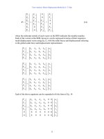
In view of Eq.15 which defines the strain energy as work done by internal forces, we can
call
δ
U as the virtual strain energy. When applying the principle of virtual force to find a
particular deflection at a point, we apply a fictitious unit load at the point of interest and
in the direction of the deflection we are to find. This unit load is the external virtual
force. The internal virtual force for a beam, corresponding to the unit load, is the bending
moment in equlibrium with the unit load and is denoted by m(x). Denoting the internal
moment induced by the real applied load as M(x), the real deformation corresponding to
the virtual moment m(x) is then
d
θ
=
EI
dxxM )(
The strain energy of an infinitesimal element is m(x)d
θ
and the integration of
m(x)d

θ
over the length of the beam gives the virtual strain energy.
δ
U = ∫ m(x)
EI
dxxM )(
The external virtual work is the product of the unit load and the deflection we want,
denoted by
∆
:
Beam and Frame Analysis: Force Method, Part II by S. T. Mau
136
δ
W = 1 (
∆
)
The principle of virtual force then leads to the following useful formula of the unit load
method.
1 (
∆
) = ∫ m(x)
EI
dxxM )(
(17)
In Eq. 17, we have indicated the linkage between the external virtual force, 1, and the
internal virtual moment, m(x), and the linkage between the real external deflection,
∆
, and
the real internal element rotation, M(x)dx/EI.
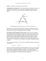
Example 16. Find the rotation and deflection at the mid-span point C of the beam shown.

EI is constant and the beam length is L.
Beam example of the unit load method.
Solution.
(1) Draw the moment diagram of the original beam problem.
Moment diagram of the original beam problem.
(2) Draw the moment diagram of the beam with a unit moment at C.
M
o
L
/2
L
/2
C
M
o
M
(x)
Beam and Frame Analysis: Force Method, Part II by S. T. Mau
137
Moment diagram of the beam under the first unit load.
(3) Compute the rotation at C.
1 (
θ
c
) = ∫ m
1
(x)
EI
dxxM )(
= 1 (

EI
M
o
) (
2
L
)=1
2EI
LM
o
radian
(
θ
c
) =
2EI
LM
o
radian.
(4) Draw the moment diagram of the beam with a unit force at C.
Moment diagram of the beam under the second unit load.
(5) Compute the deflection at C.
1 (
∆
c
) = ∫ m
2
(x)
EI
dxxM )(

= 1(
2
1
) (−
2
L
) (
EI
M
o
) (
2
L
)=1(−
EI
LM
8

2
o
)
(
∆
c
) = −
EI
LM
8

2

o
m. Upward.
C
1 kN-m
1 kN-m
L
/2
L
/2
C
1 kN
−
L/2
L
/2
m
1
(x)
m
2
(x)
L
/2
Beam and Frame Analysis: Force Method, Part II by S. T. Mau
138
In the last integration, we have used a shortcut. For simple polynomial functions, the
following table is easy to remember and easy to use.
Integration Table for Integrands as a Product of Two Simple Functions
Case (1) (2) (3) (4)
f

1
(x)
f
2
(x)
∫
L
o
dxff
21
2
1
a b L
3
1
a b L
6
1
a b L
a b L
Example 17. Find the deflection at the mid-span point C of the beam shown. EI is
constant and the beam length is L.
Example problem to find deflection at mid span.
Solution. The solution is presented in a series of figures below.
Solution to find deflection at mid span.
a
b b
a
a
a

b
b
L
/2
L
/2
C
M
o
= 1 kN-m
1 kN-m
L
/2
L
/2
C
1 kN
L
/4 kN-m
0.5
M
(x)
m(x)
B
A
Beam and Frame Analysis: Force Method, Part II by S. T. Mau
139
The computing is carried out using the integration table as a shortcut. The large triangular
shaped functions in M(x) is broken down into two triangles and one rectangle as indicated
by the dashed lines in order to apply the formulas in the table.

.
1 (
∆
c
) = ∫ m(x)
EI
dxxM )(
=(
EI
1
)[(
3
1
) (
2
1
) (
4
L
)(
2
L
) +(
2
1
) (
2
1
) (
4

L
) (
2
L
)+(
6
1
) (
2
1
) (
4
L
)(
2
L
) ]
∆
c
=
EI
L
2
16
m. Downward.
Example 18. Find the rotation at the end point B of the beam shown. EI is constant and
the beam length is L.
Example problem to find rotation at end B.
Solution. The solution is presented in a series of figures below.
Solution to find the rotation at the right end.

L
/2
L
/2
C
1 kN
L
/4 kN-m
L
/2
L
/2
C
1 kN-m
1 kN-m
0.5
B
A
M
(x)
m(x)
Beam and Frame Analysis: Force Method, Part II by S. T. Mau
140
The computing is carried out using the integration table as a shortcut. The large triangular
shaped functions in m(x) is broken down into two triangles and one rectangle as indicated
by the dashed lines in order to apply the formulas in the table.
1(
θ
B
) = ∫ m(x)

EI
dxxM )(
= (
EI
1
)[(
3
1
) (
2
1
) (
4
L
)(
2
L
) +(
2
1
) (
2
1
) (
4
L
) (
2
L
)+(

6
1
) (
2
1
) (
4
L
)(
2
L
) ]
θ
B
=
EI
L
2
16
radian. Counterclockwise.
The fact that the results of the last two examples are identical prompts us to look into the
following comparison of the two computational processes.
Side by side comparison of the two processes in Examples 17 and 18.
It is clear from the above comparison that the roles of M(x) and m(x) are reversed in the
two examples. Since the integrands used to compute the results are the product of M(x)
and m(x) and are identical, no wonder the results are identical in their numerical values.
We can identify the deflection results we obtained in the two examples graphically as
shown below.
L
/2

L
/2
C
M
o
= 1 kN-m
L
/2
L
/2
C
1 kN
0.5
L
/4 kN-m
L
/2
L
/2
C
L
/2
L
/2
C
1 kN-m
0.5
1 kN
M
o

= 1 kN-m
1 kN-m
L
/4 kN-m
M
(x)
m(x)
Beam and Frame Analysis: Force Method, Part II by S. T. Mau
141
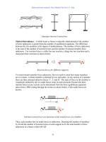
Reciprocal deflections.
We state that the deflection at C due to a unit moment at B is numerically equal to the
rotation at B due to a unit force at C. This is called the Maxwell’s Reciprocal Law,
which may be expressed as:
δ

ij
=
δ

ji
(18)
where
δ
ij
= displacement at i due to a unit load at j, and
δ
ji
= displacement at j due to a unit load at i.
The following figure illustrates the reciprocity further.
Illustration of the reciprocal theorem.

Example 19. Find the vertical displacement at point C due to a unit applied load at a
location x from the left end of the beam shown. EI is constant and the length of the beam
is L.
L
/2
L
/2
C
M
o
= 1 kN-m
L
/2
L
/2
C
1 kN
θ
B
∆
c
1 kN
1 kN
i
i
j
j
δ
ij
δ

ji
Beam and Frame Analysis: Force Method, Part II by S. T. Mau
142
Find deflection at C as a function of the location of the unit load, x.
Clearly the deflection at C is a function of x, which represents the location of the unit
load. If we plot this function against x, then a diagram or curve is established. We call
this curve the influence line of deflection at C. We now show that the Maxwell’s
reciprocal law is well suited to find this influence line for deflections.
According to the Maxwell’s reciprocal law, the deflection at C due to a unit load at x is
equal to the deflection at x due to a unit load at C. A direct application of Eq. 18 yields
δ

cx
=
δ

xc
The influence line of deflection at C is
δ

cx
, but it is equal in value to
δ

xc
which is simply
the deflection curve of the beam under a unit load at C. By applying the Maxwell’s
reciprocal law, we have transformed the more difficult problem of finding deflection for a
load at various locations to a simpler problem of find deflection of the whole beam under
a fixed unit load.

Deflection of the beam due to a unit load at C.
We can use the conjugate beam method to find the beam deflection. Readers are
encouraged to find the moment (deflection) diagram from the conjugate beam.
a
x
C
1 kN
a
x
C
1 kN
Beam and Frame Analysis: Force Method, Part II by S. T. Mau
143
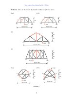
Problem 4. EI is constant in all cases. Use the unit load method in all problems.
(1) Find the deflection at point C.
(2) Find the sectional rotation at point B.
(3) Find the deflection at point B.
(4) Find the sectional rotation at point C.
(5) Find the deflection and sectional rotation at point C.
Problem 4.
L
/2
L
/2
1 kN-m
L
/2
L
/2
1 kN

L
/2
L
/2
M
o
= 1 kN-m
L
/2
L
/2
1 kN
2aaa
2Pa
C
B
B
C
C
Beam and Frame Analysis: Force Method, Part II by S. T. Mau
144
Sketch the Deflection Curve. Only the conjugate beam method gives the deflection
diagram. The unit load method gives deflection at a point. If we wish to have an idea on
how the deflection curve looks like, we can sketch a curve based on what we know about
the moment diagram.
Eq. 7 indicates that the curvature of a deflection curve is proportional to the moment.
This implies that the curvature varies in a similar way as the moment varies along a beam
if EI is constant. At any location of a beam, the correspondence between the moment and
the appearance of the deflection curve can be summarized in the table below. At the point
of zero moment, the curvature is zero and the point becomes an inflection point.

Sketch Deflection from Moment
Moment Deflection
Example 20. Sketch the deflection curve of the beam shown. EI is constant and the beam
length is L.
Beam example on sketching the deflection.
Solution. The solution process is illustrated in a series of figures shown below.
3 m
3 m
1 m
6 kN
1 kN/m
A
B
C
D
Beam and Frame Analysis: Force Method, Part II by S. T. Mau
145
Sketching a deflection curve.
Frame Deflection. The unit load method can be applied to rigid frames by using Eq. 17
and summing the integration over all members.
1 (
∆
) = ∑ ∫ m(x)
EI
dxxM )(
(17)
Within each member, the computation is identical to that for a beam.
3 m
3 m
1 m

6 kN
1 kN/m
A
B
C
D
2.5 kN
9.5 kN
2.5 kN
−3.5 kN
6.0 kN
2.5 m
V
0.125 kN-m
2 m
M
6 kN-m
3 m
3 m
3 m
1 m
A
B
C
D
I
nflection Point
3 kN-m
L
ocal max.

Beam and Frame Analysis: Force Method, Part II by S. T. Mau
146
Example 21. Find the horizontal displacement at point b.
Frame example to find displacement at a point.
Solution.
(1) Find all reactions and draw the moment diagram M of the entire frame.
ΣM
a
=0 R
dV
=2P
ΣM
d
=0 R
aV
=2P
ΣF
x
=0 R
aH
=P
Reaction and moment diagrams of the entire frame.
(2) Place unit load and draw the corresponding moment diagram m.
a
d
b
L
2L
2EI
E

I
E
I
P
a
d
b
c
L
2L
2EI
E
I
E
I
P
R
aH
R
aV
R
dV
M
2PL
c
Beam and Frame Analysis: Force Method, Part II by S. T. Mau
147
Moment diagram corresponding to a unit load.
(3) Compute the integration member by member.
Member a~b ∫m

EI
M
dx = (
EI
1
)(
3
1
) (2L) (2PL)(2L) =
3EI
PL
3
8
Member b~c ∫m
EI
M
dx = (
2EI
1
)(
3
1
) (2L) (2PL)(L) =
3EI
PL
3
2
Member c~d ∫m
EI
M

dx = 0
(4) Sum all integration to obtain the displacement.
1 (
∆
b
) = ∑ ∫ m(x)
EI
dxxM )(
=
EI
PL
3
8
3
+
EI
PL
3
2
3
=
EI
0PL
3
1
3
∆
b
=
EI

0PL
3
1
3
to the right.
Example 22. Find the horizontal displacement at point d and the rotations at b and c.
L
2L
1
1
2
2
2L
m
Beam and Frame Analysis: Force Method, Part II by S. T. Mau
148
Example problem to find displacement and rotation.
Solution. This the same problem as that in Example 20. Instead of finding
∆
b
, now we
need to find
θ
b
,
θ
c
, and
∆
d

. We need not repeat the solution for M, which is already
obtained. For each of the three quantities, we can place the unit load as shown in the
following figure.

Placing unit loads for
θ
b
,
θ
c
, and
∆
d
.
The computation process, including the reaction diagram, moment diagram for m and
integration can be tabulated as shown below. In this table, the computation in Example
20 is also included so that readers can see how the tabulation is done.
a
d
b
L
2L
2EI
E
I
E
I
P
b
a

d
c
1
b
a
d
c 1
a
d
b
c
1
f
or
θ
b
f
or
θ
c
f
or
∆
d
c
Beam and Frame Analysis: Force Method, Part II by S. T. Mau
149
Computation Process for Four Different Displacements
Actual Load Load for
∆

b
Load for
θ
b
Load for
θ
c
Load for
∆
d
Load
Diagram
Moment
Diagram
(M)(m)(m)(m)(m)
a~b
EI
1
(
3
1
)
(2PL)(2L)(2L)
=
EI
PL
3
8
3
00

EI
1
(
3
1
)
(2PL)(2L)(2L)
=
EI
PL
3
8
3
b~c
EI2
1
(
3
1
)
(2PL)(2L)(L)
=
EI
PL
3
2
3
EI2
1
(

3
1
)
(2PL)(1)(L)
=
EI
PL
3
2
EI2
1
(
6
1
)
(2PL)(1)(L)
=
EI
PL
6
2
EI2
1
(
2
1
)
(2PL)(2L)(L)
=
EI

PL
3
∫ m
EI
Mdx
c~d 0000
Σ∫ m
EI
Mdx
∆
b
=
EI
PL
3
10
3
θ
b
=
EI
PL
3
2
θ
c
=
EI
PL
6

2
∆
d
=
EI
PL
3
11
3
Knowing the rotation and displacement at key points, we can draw the displaced
configuration of the frame as shown below.
Displaced configuration.
P
2P
2P
P
1
2
2
1
1
1/L1/L
1
1/L
1/L
1
1
2PL
2L
1

1
2L
2L
P
Beam and Frame Analysis: Force Method, Part II by S. T. Mau
150
Example 23. Find the horizontal displacement at point b and the rotation at b of member
b~ c.
Frame example for finding rotation at a hinge.
Solution. It is necessary to specify clearly that the rotation at b is for the end of member
b~c, because the rotation at b for member a~b is different. The solution process is
illustrated in a series of figures below.
Drawing moment diagrams.
L
L
L
P
a
b
c
d
2EI
E
I
E
I
a
b
b
c

d
P
P
/2
P
/2
P
/2
P
/2
L
L
L
a
b
c
d
P
L/2
M
a
b
c
d
1/2
1/2
L
L
L
a

b
c
d
−L
m
L
L
L
a
b
c
d
m
1
1
−L
a
b
c
d
1/2
1/2
1
1
Beam and Frame Analysis: Force Method, Part II by S. T. Mau
151
Computation Process for a Displacement and a Rotation
Actual Load
Load for
∆

b
Load for
θ
b
Load
Diagram
Moment
Diagram
(M)(m)(m)
a~b 00
b~c
EI2
1−
[ (
2
PL
)(
2
L
)(L)
+
2
1
(
2
PL
)(
2
L
)(L)

+
6
1
(
2
PL
)(
2
L
)(L)]
= −
EI
PL
48
5
3
EI2
1
[
6
1
(
2
PL
)(
2
1
)(L)
+

2
1
(
2
PL
)(
2
1
)(L)
+
3
1
(
2
PL
)(
2
1
)(L)]
=
EI
PL
8
2
∫ m
EI
Mdx
c~d 00
Σ∫ m
EI

Mdx
∆
b
=−
EI
PL
48
5
3
θ
b
=
EI
PL
8
2
The displaced configuration is shown below.
Displaced configuration.
P
/2
P
/2
P
1/2 1/2
1
1/2L
1/2L
1
P
L/2

1
L
1
P
Beam and Frame Analysis: Force Method, Part II by S. T. Mau
152
Problem 5. Use the unit load method to find displacements indicated.
(1) Find the rotation at a and the rotation at d.
Problem 5-1.
(2) Find the horizontal displacement at b and the rotation at d.
Problem 5-2.
(3) Find the horizontal displacement at b and the rotation at d.
Problem 5-3.
a
d
b
L
2L
2EI
E
I
E
I
P
c
a
d
b
L
2L

2EI
E
I
E
I
c
P
L
L
L
L
P
L
a
b
c
d
2EI
E
I
E
I
153
Beam and Frame Analysis: Force Method, Part III
6. Statically Indeterminate Beams and Frames
When the number of force unknowns exceeds that of independent equilibrium equations,
the force method of analysis calls for additional conditions based on support and/or
member deformation considerations. These conditions are compatibility conditions and
the method of solution is called the method of consistent deformations.
The procedures of the method of consistent deformations are outlined below.

(1) Determine the degree(s) of redundancy, select the redundant force(s) and
establish the primary structure.
(2) Identify equation(s) of compatibility, expressed in terms of the redundant
force(s).
(3) Solve the compatibility equation(s) for the redundant force(s).
(4) Complete the solution by solving the equilibrium equations for all unknown
forces.
Example 24. Find all reaction forces, draw the shear and moment diagrams and sketch
the deflection curve. EI is constant.
Beam statically indeterminate to the first degree.
Solution.
(1) Degree of indeterminacy is one. We choose the reaction at b, R
b
, as the redundant.
The statically determinate primary structure and the redundant force.
(2) Establish the compatibility equation. Comparing the above two figures, we observe
that the combined effect of the load P and the reaction R
b
must be such that the total
L
/2
L
/2
P
a
b
P
a
b
R

b
Beam and Frame Analysis: Force Method, Part III by S. T. Mau
154
vertical displacement at b is zero, which is dictated by the roller support condition of
the original problem. Denoting the total displacement at b as
∆
b
we can expressed the
compatibility equation as
∆
b

=
∆
b
’

+ R
b
δ
bb
= 0
where
∆
b
’ is the displacement at b due to the applied load and
δ
bb
is the displacement
at b due to a unit load at b. Together, R

b
δ
bb
represents the displacement at b due to
the reaction R
b
. The combination of
∆
b
’

and R
b
δ
bb
is based on the concept of
superposition, which states that the displacement of a linear structure due to two loads
is the superposition of the displacement due to each of the two loads. This principle is
illustrated in the figure below.
Compatibility equation based on the principle of superposition.
(3) Solve for the redundant force. Clearly the redundant force is expressed by
R
b
= −

bb
b
δ
∆
'

To find
∆
b
’ and
δ
bb
, we can use the conjugate beam method for each separately, as
shown below.
P
a
b
R
b
P
a
b
a
b
R
b
R
b
δ
bb
∆
b
’
=
+
∆

b
= 0