Fundamentals of Structural Analysis Episode 2 Part 1 pdf

175
Beam and Frame Analysis: Displacement Method
Part I
1. Introduction
The basic concept of the displacement method for beam and frame analysis is that the
state of a member is completely defined by the displacements of its nodes. Once we
know the nodal displacements, the rest of the unknowns such as member forces can be
obtained easily.
For the whole structure, its state of member force is completely defined by the
displacements of its nodes. Once we know all the nodal displacements of the structure,
the nodal displacements of each member is obtained and member forces are then
computed.
Defining a node in most cases is easy; it either appears as a joining point of a beam and a
column, or it is at a location where there is a support. In other cases, it is a matter of
preference of the analyzer, who may decide to define a node anywhere in a structure to
facilitate the analysis.
We will introduce the displacement method in three stages: The moment distribution
method is introduced as an iterative solution method which does not explicitly formulate
the governing equations. The slope-deflection method is then introduced to formulate the
governing equations. Both are identical in their assumptions and concepts. The matrix
displacement method is then introduced as a generalization of the moment distribution
and slope-deflection methods.
2. Moment Distribution Method
The moment distribution method is a unique method of structural analysis, in which
solution is obtained iteratively without ever formulating the equations for the unknowns.
It was invented in an era, out of necessity, when the best computing tool was a slide rule,
to solve frame problems that normally require the solution of simultaneous algebraic
equations. Its relevance today, in the era of personal computer, is in its insight on how a
beam and frame reacts to applied loads by rotating its nodes and thus distributing the
loads in the form of member-end moments. Such an insight is the foundation of the
modern displacement method.

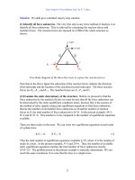
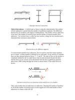
Take the very simple frame shown as an example. The externally applied moment at
node b tends to create a rotation at node b. Because member ab and member bc are
rigidly connected at node b, the same rotation must take place at the end of member ab
and member bc. For rotation at the end of member ab and member bc to happen, an end
moment must be internally applied at the member end. This member-end moment comes
from the externally applied moment. Nodal equilibrium at b requires the applied external
Beam and Frame Analysis: Displacement Method, Part I by S. T. Mau
176
moment of 100kN be distributed to the two ends of the two joining members at b. How
much each member will receive depends on how “rigid” each member is in their
resistance to rotation at b. Since the two members are identical in length, L, and cross-
section rigidity, EI, we assume for the time being that they are equally rigid. Thus, half
of the 100 kN-m goes to member ab and the other half goes to member bc.
A frame example showing member-end moments.
In the above figure, only the member-end moments are shown. The member-end shear
and axial forces are not shown to avoid overcrowding the figure. The distributed
moments are “member-end” moments denoted by M
ba
and M
bc
respectively. The sign
convention of member-end moments and applied external moments is: clockwise is
positive. We assume the two members are equally rigid and receive half of the applied
moment, not only because they appear to be equally rigid but also because each of the
two members is under identical loading conditions: fixed at the far end and hinged at the
near end.
In other cases, the beam and column may not be of the same rigidity, but they may have
the same loading and supporting conditions: fixed at the far end and allowed to rotate at
the near end. This configuration is the fundamental configuration of moment loading
100 kN-m

E
I, L
E
I, L
a
c
b
100 kN-m
50 kN-m
50 kN-m
b
E
I, L
E
I, L
a
c
b
b
50 kN-m
50 kN-m
Moment equilibrium
of node b
Beam and Frame Analysis: Displacement Method, Part I by S. T. Mau
177
from which all other configurations can be derived by the principle of superposition. We
shall delay the derivation of the governing formulas until we have learned the operating
procedures of the moment distribution method.
Beam and column in a fundamental configuration of a moment applied at the end.
Suffices it to say that given the loading and support conditions shown below, the rotation

θ
b
and member-end moment M
ba
at the near end, b, is proportional. The relationship
between M
ba
and
θ
b
is expressed in the following equation, the derivation of which will
be given later.
The fundamental case and the reaction solutions.
M
ba
= 4(EK)
ab
θ
b
, where K
ab
=(
L
I
)
ab
.(1)
We can write a similar equation for M
bc
of member bc.

M
bc
= 4(EK)
bc
θ
b
, where K
bc
=(
L
I
)
bc
.(1)
M
ba
θ
b
E
I, L
a
c
b
b
M
bc
θ
b
M
ba

=4EK
θ
b
E
I, L
a
b
θ
b
M
ba
=2EK
θ
b
V
ba
=6EK
θ
b
/L
V
ab
=6EK
θ
b
/L
Beam and Frame Analysis: Displacement Method, Part I by S. T. Mau
178
Furthermore, the moment at the far end of member ab, M
ab

at a, is related to the amount
of rotation at b by the following formula:
M
ab
= 2(EK)
ab
θ
b
(2)
Similarly, for member bc,
M
cb
= 2(EK)
bc
θ
b
(2)
As a result, the member-end moment at the far end is one half of the near end moment:
M
ab
=
2
1
M
ba
(3)
and
M
cb
=

2
1
M
bc
(3)
Note that in the above equations, it is important to keep the subscripts because each
member may have a different EK.
The significance of Eq. 1 is that it shows that the amount of member-end moment,
distributed from the unbalanced nodal moment, is proportional to the member stiffness
4EK, which is the moment needed at the near end to create a unit rotation at the near end
while the far end is fixed. Consequently, when we distribute the unbalanced moment, we
need only to know the relative stiffness of each of the joining members at that particular
end. The equilibrium equation for moment at node b is
M
ba
+ M
bc
= 100 kN-m (4)
Since
M
ba
: M
bc
= (EK)
ab
: (EK)
bc
,
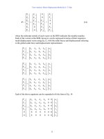
we can “normalize” the above equation so that both sides would add up to one, i.e. 100%,
utilizing the fact that (EK)

ab
= (EK)
bc
in the present case:
bcba
ab
MM
M
+
:
bcba
bc
MM
M
+

=
c
)()(
)(
bab
ab
EKEK
EK
+
:
c
)()(
)(
bab

bc
EKEK
EK
+

=
2
1
:
2
1
(5)
Consequently
M
ba
=
2
1
( M
ba
+ M
bc
) =
2
1
(100 kN-m) = 50 kN-m.
Beam and Frame Analysis: Displacement Method, Part I by S. T. Mau
179
M
bc

=
2
1
( M
ba
+ M
bc
) =
2
1
(100 kN-m) = 50 kN-m.
From Eq. 2, we obtain
M
ab
=
2
1
M
ba
= 25 kN-m.
M
cb
=
2
1
M
bc
= 25 kN-m.
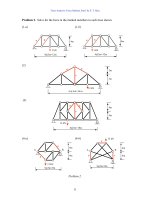
Now that all the member-end moments are obtained, we can proceed to find member-end
shears and axial forces using the FBDs below.

FBDs to find shear and axial forces.
The dashed lines indicate that the axial force of one member is related to the shear force
from the joining member at the common node. The shear forces are computed from the
equilibrium conditions of the FBDs :
V
ab
= V
ba
=
ab
abba
L
MM +
and
V
bc
= V
cb
=
bc
cbbc
L
MM +
The moment and deflection diagrams of the whole structure are shown below.
V
ab
V
ba
V
bc

V
cb
25 kN-m
25 kN-m
50 kN-m
50 kN-m
Beam and Frame Analysis: Displacement Method, Part I by S. T. Mau
180

Moment and deflection diagrams.
In drawing the moment diagram, note that the sign conventions for internal moment ( as
in moment diagram) and the member-end moment (as in Eq.1 through Eq.5) are different.
The former depends on the orientation and which face the moment is acting on and the
latter depends only on the orientation (clockwise is positive).
Difference in sign conventions.
Let us recap the operational procedures of the moment distribution method:
(1) Identify the node which is free to rotate. In the present case, it was node b. The
number of “free” rotating nodes is called the degree-of-freedom (DOF). In the present
case, the DOF is one.
(2) Identify the joining members at this node and computer their relative stiffness
according to Eq. 5, which can be generalized to cover more then two members.
xy
ab
M
M
∑
:
xy
bc
M

M
∑

:
xy
cd
M
M
∑
…

=
y
)(
)(
x
ab
EK
EK
∑
:
y
)(
)(
x
bc
EK
EK
∑

:
y
)(
)(
x
cd
EK
EK
∑
… (5)
where the summation is over all joining members at the particular node. Each of the
expression in this equation is called a distribution factor (DF), which adds up to one
or 100%. Each of the moment at the end of a member is called a member-end
moment (MEM).
(3) Identify the unbalanced moment at this node. In the present case, it was 100 kN-m.
(4) To balance the 100 kN-m, we need to add −100 kN-m to the node, which, when
viewed from the member end, becomes positive 100 kN-m. This 100 kN-m is
distributed to member ab and bc according to the DF of each member. In this case
50 kN-m
25 kN-m
25 kN-m
+
M
∆
P
ositive internal moment
P
ositive member-end moment
P
ositive internal moment

N
egative member-end moment
Beam and Frame Analysis: Displacement Method, Part I by S. T. Mau
181
the DF is 50% each. Consequently 50 kN-m goes to M
ba
and 50 kN-m goes to M
bc
.
They are called the distributed moment (DM). Note that the externally applied
moment is distributed as member-end moments in the same sign, i.e. positive to
positive.
(5) Once the balancing moment is distributed, the far ends of the joining members
should receive 50% of the distributed moment at the near end. The factor of 50% or _
is called the carryover factor (COF). The moment at the far end thus distributed is
called the carryover moment (COM). In the present case, they are 25 kN-m for M
ab
and 25 kN-m for M
cb
, respectively.
(6) We note that at the two fixed ends, whatever moments are carried over, they are
balanced by the support reaction. That means the moment equilibrium is achieved at
the fixed ends with no need for additional distribution. This is equivalent to say that
the stiffness of the support relative to the stiffness of the member is infinite. Or, even
simpler, we may formally designate the distribution factors at a fixed support as 1: 0,
where one being assigned for the support and zero assigned to the member. The zero
DF means we need not re-distributed any moment at the member-end.
(7) The moment distribution method operations end when all the nodes are in moment
equilibrium. In the present case, node b is the only node we need to concentrate on
and it is in equilibrium after the unbalanced moment is distributed.

(8) To complete the solution process, however, we still need to find the other unknowns
such as shear and axial forces at the end of each member. That is accomplished by
drawing the FBD of each member and writing equilibrium equations.
(9) The moment diagram and deflection diagram can then be drawn.
We shall now go through the solution process by solving a similar problem with a single
degree of freedom (SDOF).
Example 1. Find all the member-end moments of the beam shown. EI is constant for all
members.
Beam problem with a SDOF.
Solution.
(1) Preparation.
(a) Unbalanced moment: At node b there is an externally applied moment
(EAM), which should be distributed as member-end moments (MEM) in the
same sign.
(b) The distribution factors at node b:
30 kN-m
a
b
c
10 m
5 m
Beam and Frame Analysis: Displacement Method, Part I by S. T. Mau
182
DF
ba
: DF
bc
= 4EK
ab
: 4EK

bc
= 4(
L
EI
)
ab
: 4(
L
EI
)
bc
=
10
1
:
5
1
=
15
5
:
15
10
= 0.33 : 0.67
(c) As a formality, we also include DF
ab
=0, and DF
bc
= 0, at a and c respectively.
(2) Tabulation: All the computing can be tabulated as shown below. The arrows indicate

the destination of the carryover moment. The dashed lines show how the distribution
factor (DF) is used to compute the distributed moment (DM).
Moment Distribution Table for a SDOF Problem
Node ab c
Member ab bc
DF 0 0.33 0.67 0
MEM
1
M
ab
M
ba
M
bc
M
cb
EAM
2
30
DM
3
+10 +20
COM
4
+5 +10
Sum
5
+5 +10 +20 +10
1. Member-end-moment.
2. Externally applied moment.

3. Distributed member-end-moment.
4. Carry-over-moment.
5. Sum of member-end-moments.
(3) Post Moment-Distribution Operations. The moment and deflection diagrams are
shown below.
Moment and deflection diagrams.
The moment distribution method becomes iterative when there are more than one DOF.
The above procedures for one DOF problem can still apply if we consider one DOF at a
time. That is to say that when we concentrate on one DOF, the other DOFs are considered
“locked” into a fixed support and not allow to rotate. When the free node gets its
distributed moment and the carryover moment reaches the neighboring and previously
locked node, that node becomes unbalanced, thus requiring “unlocking” to distribute the
balancing moment, which in turn creates carryover moment at the first node. That
requires another round of distribution and carrying over. Thus begins the cycle of
“locking-unlocking” and the balancing of moments from one node to another. We shall
20 kN-m
−10 kN-m−10 kN-m
5 kN-m
I
nflection point
Beam and Frame Analysis: Displacement Method, Part I by S. T. Mau
183
see, however, in each subsequent iteration, the amount of unbalanced moment becomes
progressively smaller. The iteration stops when the unbalanced moment becomes
negligible. This iterative process is illustrated in the following example of two DOFs.
Example 2. Find all the member-end moments of the beam shown. EI is constant for all
members.
Example of a beam with two DOFs.
Solution.
(1) Preparation.

(a) Both nodes b and c are free to rotate. We choose to balance node c first.
(b) Compute DF at b:
DF
ba
: DF
bc
= 4EK
ab
: 4EK
bc
= 4(
L
EI
)
ab
: 4(
L
EI
)
bc
=
3
1
:
5
1
= 0.625 : 0.375
(c) Compute DF at c:
DF
cb

: DF
cd
= 4EK
bc
: 4EK
cd
= 4(
L
EI
)
bc
: 4(
L
EI
)
cd
=
5
1
:
5
1
= 0.5 : 0.5
(d) Assign DF at a and d: DFs are zero at a and d.
(2) Tabulation
3m 5m 5m
a
b
c
d

30 kN-m
Beam and Frame Analysis: Displacement Method, Part I by S. T. Mau
184
Moment Distribution for a Two-DOF Problem
Node ab cd
Member ab bc cd
DF 0 0.625 0.375 0.5 0.5 0
MEM M
ab
M
ba
M
bc
M
cb
M
cd
M
dc
EAM 30
DM +15 +15
COM +7.50 +7.50
DM −4.69 −2.81
COM −2.35 −1.41
DM +0.71 +0.70
COM +0.36 0.35
DM −0.22 −0.14
COM −0.11 −0.07
DM +0.04 +0.03
COM +0.02 +0.02

DM −0.01 −0.01
COM 0.00 0.00
SUM −2.46 −4.92 +4.92 +14.27 +15.73 +7.87
In the above table, the encircled moment is the unbalanced moment. Note how the
circles move back and forth between nodes b and c. Also note how the externally applied
moment (EAM) at c and the unbalanced moment, created by the carried over moment
(COM) at b are treated differently. The EAM is balanced by distributing the amount in
the same sign to the member ends, while the unbalanced moment at a node is balanced by
distributing the negative of the unbalanced moment to the moment ends.
(3) Post Moment-Distribution Operations. The moment and deflection diagrams are
shown below.
Moment and deflection diagrams.
Treatment of load between nodes. In the previous examples, the applied load was an
applied moment at a node. We can begin the distribution process right at the node. In
most practical cases, the load will be either concentrated loads or distributed loads
−2.46
4.92
-14.27
15.73
-7.87
I
nflection point
Beam and Frame Analysis: Displacement Method, Part I by S. T. Mau
185
applied between nodes. These cases call for an additional step before we can begin the
distribution of moments.
Load applied between nodes.
We imagine that all the nodes are “locked” at the beginning. Then each member is in a
state of a clamped beam with transverse load applied between the two ends.
Fixed-end beam with applied load.

The moment needed to “lock” the two ends are called fixed-end moments(FEM). They
are positive if acting clockwise. For typical loads, the FEMs can be pre-computed and
are tabulated in the fixed-end moment table given at the end of this unit. These FEMs are
to be balanced when the node is “unlocked” and allowed to rotate. Thus, the effect of the
transverse load applied between nodes is to create moments at both ends of a member.
These FEMs should be balanced by moment distribution.
Example 3. Find all the member-end moments of the beam shown. EI is constant for all
members.
Example with load applied between nodes.
Solution.
(1) Preparation.
(a) Only nodes b is free to rotate. There is no externally applied moment at node b
to balance, but the transverse load between nodes create FEMs.
(b) FEM for member ab. The concentrated load of 4 kN creates FEMs at end a
and end b. The formula for a single transverse load in the FEM table gives us:
a
b
M
F
ba
M
F
ab
2 m
2 m 4 m
a
c
b
3 kN/m
4 kN

P
Beam and Frame Analysis: Displacement Method, Part I by S. T. Mau
186
M
F
ab
= −
8
)( )( LengthP
= −
8
(4) (4)
= − 2 kN-m
M
F
ba
=
8
)( )( LengthP
=
8
(4) (4)
= 2 kN-m
(c) FEM for member bc. The distributed load of 3 kN/m creates FEMs at end b
and end c. The formula for a distributed transverse load in the FEM table
gives us:
M
F
bc
= −

12
)( )(
2
Lengthw
= −
12
(4) (3)
2
= − 4 kN-m
M
F
cb
=
12
)( )(
2
Lengthw
=
12
(4) (3)
2
= 4 kN-m
(d) Compute DF at b:
DF
ba
: DF
bc
= 4EK
ab
: 4EK

bc
= 4(
L
EI
)
ab
: 4(
L
EI
)
bc
=
4
1
:
4
1
= 0.5 : 0.5
(e) Assign DF at a and c: DFs are zero at a and c.
(2) Tabulation.
Moment Distribution for a SDOF Problem with FEMs
Node abc
Member ab bc
DF 0 0.5 0.5 0
EAM
MEM M
ab
M
ba
M

bc
M
cb
FEM −2+2−4+4
DM +1 +1
COM +0.5 +0.5
Sum −1.5 +3 −3 +4.5
(3) Post Moment-Distribution Operations. The shear forces at both ends of a member are
computed from the FBDs of each member. Knowing the member-end shear forces,
the moment diagram can then be drawn. The moment and deflection diagrams are
shown below.
FBDs of the two members.
1.5 kN-m
2 m
2 m
4 kN
3 kN-m
2.38 kN
1.62 kN
3 kN-m
4 m
3 kN/m
4.5 kN-m
6.38 kN
5.62 kN
Beam and Frame Analysis: Displacement Method, Part I by S. T. Mau
187
Moment and deflection diagrams.
Treatment of Hinged Ends. At a hinged end, the member-end moment (MEM) is equal
to zero or whatever an externally applied moment is at the end. During the process of

moment distribution, the hinged end may receive carried-over moment from the
neighboring node. That COM must then be balanced by distributing 100% of it at the
hinged end. This is because the distribution factor of a hinged end is one or 100%; the
hinged end maybe considered to be connected to air which has zero stiffness. This new
distributed moment starts another cycle of carrying-over and distribution. This process is
illustrated in Example 4.
The cycle of iteration is greatly simplified if we recognize at the very beginning of
moment distribution that the stiffness of a member with a hinged end is fundamentally
different from that of the standard model with the far end fixed. We will delay the
derivation but will state that the moment needed at the near end to create a unit rotation at
the near end with the far end hinged is 3EK, less than the 4EK if the far end is fixed.
Member with a hinged end vs. the standard model with the far end fixed.
Note that there is no carry-over-moment at the hinged end (M
ba
= 0) if we take the
member stiffness factor as 3EK instead of 4EK. We can thus compute the relative
distribution factors accordingly and when distribute the moment at one end of the
member, need not carryover the distributed moment to the hinged end. This simplified
process with a modified stiffness from 4EK to 3EK is illustrated in Example 5.
Example 4. Find all the member-end moments of the beam shown. EI is constant for all
members.
M
ba
= 3EK
θ
b
θ
b
θ
b

M
ba
= 4EK
θ
b
M
ab
= 2EK
θ
b
M
ba
= 0
−1.5
−3
−4.5
1.75
5.79
1.875m
a
a
b
b
I
nflection point
Beam and Frame Analysis: Displacement Method, Part I by S. T. Mau
188
Turning a problem with a cantilever end into one with a hinged end.
Solution. The original problem with a cantilever end can be treated as one with a hinged
end as shown. We shall solve only the problem with a hinged end. Note that the vertical

load is not shown in the equivalent hinged-end problem because it is taken up by the
support at a.
(1) Preparation. Since the geometry and loading are similar to that of Example 3, we can
copy the preparation part but note that an externally applied moment is present.
(a) Only nodes b is free to rotate. There is an externally applied moment at node a
and the transverse load between nodes create FEMs at all nodes.
(b) FEM for member ab. The concentrated load of 4 kN creates FEMs at end a
and end b. The formula for a single transverse load in the FEM table gives us:
M
F
ab
= −
8
)( )( LengthP
= −
8
(4) (4)
= − 2 kN-m
M
F
ba
=
8
)( )( LengthP
=
8
(4) (4)
= 2 kN-m
(c) FEM for member bc. The distributed load of 3 kN/m creates FEMs at end b
and end c. The formula for a distributed transverse load in the FEM table

gives us:
M
F
bc
= −
12
)( )(
2
Lengthw
= −
12
(4) (3)
2
= − 4 kN-m
M
F
cb
=
12
)( )(
2
Lengthw
=
12
(4) (3)
2
= 4 kN-m
(d) Compute DF at b:
2 m
2 m

4 m
a
c
b
3 kN/m
4 kN
2 m
2 kN
2 m
2 m
4 m
a
c
b
3 kN/m
4 kN
4 kN-m
Beam and Frame Analysis: Displacement Method, Part I by S. T. Mau
189
DF
ba
: DF
bc
= 4EK
ab
: 4EK
bc
= 4(
L
EI

)
ab
: 4(
L
EI
)
bc
=
4
1
:
4
1
= 0.5 : 0.5
(e) Assign DF at a and c: DFs are one at a and zero c.
(2) Tabulation. In the moment distribution process below, we must deal with the
unbalanced moment at the hinged end first. The EAM of –4 kN-m and the FEM of
–2 kN-m at node a add up to 2 kN-m of unbalanced moment, not –6 kN-m. This is
because the FEM and distributed moment (DM) at node a should add up to the EAM,
which is –4 kN-m. Thus we need to distribute (–4 kN-m) – (–2 kN-m)= –2 kN-m. to
make the node balanced. The formula to remember is DM=EAM–FEM. This formula
is applicable to all nodes where there are both EAMs and FEMs.
Moment Distribution Table for a Beam with a Hinged End
Node abc
Member ab bc
DF 1 0.5 0.5 0
MEM M
ab
M
ba

M
bc
M
cb
EAM −4
FEM −2+2−4+4
DM −2
COM −1
DM +1.5 +1.5
COM +0.8 +0.8
DM -0.8
COM −0.4
DM +0.2 +0.2
COM +0.1 +0.1
DM −0.1
COM 0.0
Sum −4 +2.3 −2.3 +4.9
The above back-and-forth iteration between nodes a and b is avoided if we use the
simplified procedures as illustrated below.
Example 5. Find all the member-end moments of the beam shown. EI is constant for all
members. Use the modified stiffness to account for the hinged end at node a.
Beam with a hinged end.
2 m
2 m
4 m
a
c
b
3 kN/m
4 kN

4 kN-m
Beam and Frame Analysis: Displacement Method, Part I by S. T. Mau
190
Solution.
(1) Preparation. Note the stiffness computation in step (d).
(a) Only node b is free to rotate. There is an externally applied moment at node a
and the transverse load between nodes create FEMs at all nodes.
(b) FEM for member ab. The concentrated load of 4 kN creates FEMs at end a
and end b. The formula for a single transverse load in the FEM table gives us:
M
F
ab
= −
8
)( )( LengthP
= −
8
(4) (4)
= − 2 kN-m
M
F
ba
=
8
)( )( LengthP
=
8
(4) (4)
= 2 kN-m
(c) FEM for member bc. The distributed load of 3 kN/m creates FEMs at end b

and end c. The formula for a distributed transverse load in the FEM table
gives us:
M
F
bc
= −
12
)( )(
2
Lengthw
= −
12
(4) (3)
2
= − 4 kN-m
M
F
cb
=
12
)( )(
2
Lengthw
=
12
(4) (3)
2
= 4 kN-m
(d) Compute DF at b:
DF

ba
: DF
bc
= 3EK
ab
: 4EK
bc
= 3(
L
EI
)
ab
: 4(
L
EI
)
bc
=
7
3
:
7
4
= 0.43 : 0.57
(e) Assign DF at a and c: DFs are one at a and zero c.
(2) Tabulation. In the moment distribution process below, we must deal with the
unbalanced moment at the hinged end first. Using the formula DM=EAM–FEM, we
begin by distributing –2 kN-m and carrying over half of it to node b. From this point
on, node a is balanced, will not receive any carry-over-moment from node b, and will
stay balanced throughout the moment distribution process. The zero COM at node a

in the table below serves to emphasize there is no carrying-over.
Beam and Frame Analysis: Displacement Method, Part I by S. T. Mau
191
Moment Distribution Table for a Problem with a Hinged End
Node abc
Member ab bc
DF 0 0.43 0.57 0
MEM M
ab
M
ba
M
bc
M
cb
EAM -4
FEM -2+2-4+4
DM -2
COM -1
DM +1.3 +1.7
COM 0.0 +0.8
SUM -4.0 +2.3 -2.3 +4.8
(3) Post Moment-Distribution Operations. The moment and deflection diagrams are
shown below.
Moment and deflection diagrams.
Treatment of a Central-Symmetric or Anti-Symmetric Span. In a problem with at
least three spans, if the geometry and stiffness are symmetric about the center line of the
structure, then the central span is in (a) a state of symmetry if the load is symmetric about
the center line, and (b) a state of anti-symmetry if the load is anti-symmetric about the
center line. For these special spans, we can develop special stiffness formulas so that no

carry-over is needed across the line of symmetry when member-end moments are
distributed. The basic information needed for moment distribution is shown in the figure
below.
Symmetric and anti-symmetric spans.
We shall delay the derivation of the stiffness formulas but will simply state that for a
symmetric span, the moments needed at both ends to create a unit rotation at both ends
M
cb
= 2EK
θ
c
M
bc
= 2EK
θ
b
M
cb
= 6EK
θ
c
M
bc
= 6EK
θ
b
−4
−2.3
−4.8
0.85

2.52
1.79m
I
nflection point
b
c
θ
b
=−
θ
c
θ
b
=
θ
c
b
c
Beam and Frame Analysis: Displacement Method, Part I by S. T. Mau
192
are 2EK, and for an anti-symmetric span they are 6EK. The two examples below will
illustrate the solution processes using these modified stiffness factors. Because of
symmetry/anti-symmetry, we need to deal with only half of the span. The other half is a
mirror image of the first half in the case of symmetry and an upside down mirror image
in the case of anti-symmetry.
Example 6. Find all the member-end moments of the beam shown. EI is constant for all
members. Use the modified stiffness to account for the symmetric span between nodes b
and c.
Beam with a symmetric central span.
Solution.

(1) Preparation. Note the stiffness computation in step (c).
(a) Only nodes b and c are free to rotate. Only the transverse load between nodes
b and c will create FEMs at b and c.
(b) FEM for member bc. The formula for a single transverse load in the FEM
table gives us, as in Example 5:
M
F
bc
= − 2 kN-m
M
F
cb
= 2 kN-m
(c) Compute DF at b:
DF
ba
: DF
bc
= 4EK
ab
: 2EK
bc
= 4(
L
EI
)
ab
: 2(
L
EI

)
bc
=
6
4
:
6
2
= 0.67 : 0.33
(d) Assign DF at a: DF is one at a. No need to consider node d.
(2) Tabulation. In the moment distribution process below, we need to deal with only half
of the beam. There is no carry-over moment from b to c. We include node c just to
illustrate that all its moments are the reflection of those at node b.
2 m
2 m
4 m
a
d
b
4 kN
c
4 m
Beam and Frame Analysis: Displacement Method, Part I by S. T. Mau
193
Moment Distribution Table for a Symmetric Problem
Node abc
Member ab bc
DF 0 0.67 0.33 0
MEM M
ab

M
ba
M
bc
M
cb
EAM
FEM -4 +4
DM +2.67 +1.33 −1.33
COM +1.33
SUM +1.33 +2.67 −2.67 +2.67
(3) Post Moment-Distribution Operations. The moment and deflection diagrams are
shown below.
Moment and deflection diagrams.
Example 7. Find all the member-end moments of the beam shown. EI is constant for all
members. Use the modified stiffness to account for the anti-symmetric span between
nodes b and c.
Beam with a central anti-symmetric span.
Solution.
(1) Preparation. Note the stiffness computation in step (c). There is no need for node c.
(a) Only nodes b and c are free to rotate. The transverse load between nodes a
and b will create FEMs at a and b. No need to consider member cd.
(b) FEM for member ab. The formula for a single transverse load in the FEM
table gives us, as in Example 5 with the signs reversed:
M
F
ab
= 2 kN-m
M
F

bc
= −2 kN-m
2 m
2 m
4 m
a
d
b
4 kN
c
2 m2 m
4 kN
1.33
1.33
1.33
−2.67
−2.67
I
nflection point
Beam and Frame Analysis: Displacement Method, Part I by S. T. Mau
194
(c) Compute DF at b:
DF
ba
: DF
bc
= 4EK
ab
: 6EK
bc

= 4(
L
EI
)
ab
: 6(
L
EI
)
bc
=
10
4
:
10
6
= 0.4 : 0.6
(d) Assign DF at a: DF is one at a. No need to consider node d.
(2) Tabulation. In the moment distribution process below, we need to deal with only half
of the beam. There is no carry-over moment from b to c.
Moment Distribution Table for a Beam with an Anti-symmetric Span
Node abc
Member ab bc
DF 0 0.4 0.6 0
MEM M
ab
M
ba
M
bc

M
cb
EAM
FEM +2 −2
DM +0.8 +1.2 1.2
COM +0.4
SUM +0.4 −1.2 +1.2 +1.2
(3) Post Moment-Distribution Operations. The moment and deflection diagrams are
shown below.
Moment and deflection diagrams.
While the anti-symmetric loading seems improbable, it often is the result of
decomposition of a general loading pattern applied to a symmetrical structure. It is
always possible to decompose a general loading pattern applied on a symmetric structure
into a symmetric component and an anti-symmetric component as illustrated below.
Each loading component can then be treated with the simplified procedure of the moment
distribution method. The results of the two analyses are then superposed to obtain the
solution for the original loading pattern.
Decompose a load into a symmetric component and an anti-symmetric component.
Example 8. Find all the member-end moments of the frame shown.
0.4
1.2
−3.8
3.8
−0.4
−1.2
I
nflection point
P
P
/2

P
/2
P
/2
P
/2
=
+