Fundamentals of Structural Analysis Episode 2 Part 6 doc

Other Topics by S. T. Mau
275
Moment-rotation formulas for non-prismatic members—member rotation.
Using the identity in Eq. 1 the moment rotation formulas can be recast as:
M
ab
= −S
ab
(1+C
ab
)
φ
ab
(2)
M
ba
= −S
ba
(1+C
ba
)
φ
ab
(2)
Combining the above formulas, we can write the moment-rotation formulas for a non-
prismatic member as:
M
ab
= S
ab
θ

a
+ C
ba
S
ba
θ
b
−S
ab
(1+C
ab
)
φ
ab
+M
F
ab
(3)
M
ba
= C
ab
S
ab
θ
a
+ S
ba
θ
−S

ba
(1+C
ba
)
φ
ab
+ M
F
ba
(3)
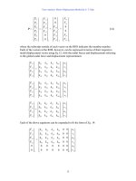
These two equations are to be used in any displacement method of analysis. A sample of
the numerical values of the factors in these two equations is given in the table below for
two configurations of rectangular sections. The EK in the table refers to the EK
calculated from the least sectional dimension of the member.
φ
M
ba
=6EK
φ
a
b
E
I,L
φ
M
ab
=6EK
φ
φ
M

ba
=−(S
ba
+C
ab
S
ab
)
φ
a
b
E
I,L
φ
M
ab
=−(S
ab
+C
ba
S
ba
)
φ
P
rismatic members
N
on-prismatic members
Other Topics by S. T. Mau
276

Stiffness and Carryover Factors and Fixed-End Moments
C
ab
C
ba
S
ab
S
ba
M
F
ab
M
F
ba
M
F
ab
M
F
ba
0.691 0.691 9.08EK 9.08EK
-0.159PL 0.159PL -0.102wL
2
0.102wL
2
C
ab
C
ba

S
ab
S
ba
M
F
ab
M
F
ba
M
F
ab
M
F
ba
0.694 0.475 4.49EK 6.57EK
-0.097PL 0.188PL -0.067wL
2
0.119wL
2
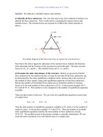
Example 1. Find all the member-end moments of the beam shown. L=10 m.
Non-prismatic beam example.
Solution. We choice to use the slope-deflection method. There is only one DOF, the
rotation at node b:
θ
b
.
The equation of equilibrium is:
Σ M

b
= 0 M
ba
+ M
bc
= 0
The EK based on the minimum depth of the beam, h, is the same for both members.
The fixed-end moments are obtained from the above table:
P
L
/2
L
/2
w
L
L
/2
L
/2
L
0.2L0.2L 0.6L
h
h
b
a
0.2L0.8L
h
h
b
a

0.2L0.2L 0.3L
c
0.2L0.8L
h
h
b
a
h
h
0.3L
100 kN
10 kN/m
w
P
Other Topics by S. T. Mau
277
For member ab: M
F
ab
= −0.067 wL
2
= −67 kN-m
M
F
ba
= 0.119 wL
2
= 119 kN-m
For member bc: M
F

bc
= −0.159 PL= −159 kN-m
M
F
cb
= 0.159 PL = 159 kN-m
The moment-rotation formulas are:
M
ba
= C
ab
S
ab
θ
a
+ S
ba
θ
b
+ M
F
ba
= 6.57EK
θ
b
+ 119
M
bc
= S
bc

θ
b
+ C
cb
S
cb
θ
c
+ M
F
bc
= 9.08EK
θ
b
− 159
The equilibrium equation M
ba
+ M
bc
= 0 becomes
15.65EK
θ
b
– 40 = 0 EK
θ
b
= 2.56 kN-m
Substituting back to the member-end moment expressions, we obtain
M
ba

= 6.57EK
θ
b
+ 119= 135.8 kN-m
M
bc
= 9.08EK
θ
b
− 159= −135.8 kN-m
For the other two member-end moments not involved in the equilibrium equation, we
have
M
ab
= C
ba
S
ba
θ
b
+M
F
ab
= (0.475)(6.57EK)
θ
b
-67 = −59.0 kN-m
M
cb
= C

bc
S
bc
θ
b
+ M
F
bc
= (0.691)(9.08EK)
θ
b
+ 159= 175.0 kN-m
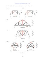
Problem 1.
(1) Find the reaction moment at support b. L=10 m.
Problem 1. (1)
0.2L0.8L
h
b
a
10 kN/m
h
Other Topics by S. T. Mau
278
(2) Find the reaction moment at support c. L=10 m.
Problem 1. (2)
3. Support Movement, Temperature, and Construction Error
Effects
A structure may exhibit displacement or deflection from its intended configuration for
causes other than externally applied loads. These causes are support movement,
temperature effect and construction errors. For a statically determinate structure, these

causes will not induce internal stresses because the members are free to adjust to the
change of geometry without the constraint from supports or from other members. In
general, however, internal stresses will be induced for statically indeterminate structures.
Statically determinate and indeterminate structures react differently to settlement.
Support Movement. For a given support movement or settlement, a structure can be
analyzed with the displacement method as shown in the following example.
Example 2. Find all the member-end moments of the beam shown. The amount of
settlement at support b is 1.2 cm, downward. EI=24,000 kN- m
2
.
A beam with a downward settlement at support b.
R
igid-body rotation without stress
D
eformed beam with stress
6 m 4 m
a
b
c
1.2 cm
0.2L0.8L
h
b
a
10 kN/m
h
0.5L
c
Other Topics by S. T. Mau
279

Solution. We shall use the slope-deflection method. The downward settlement at support
b causes member ab and member bc to have member rotations by the amount shown
below:
φ
ab
= 1.2 cm/6 m=0.002 rad.
φ
bc
= −1.2 cm/4 m= −0.003 rad.
There is only one unknown, the rotation at node b:
θ
b
.
The equation of equilibrium is:
Σ M
b
= 0 M
ba
+ M
bc
= 0
The stiffness factors of the two members are :
EK
ab
= 4,000 kN-m and EK
bc
= 6,000 kN-m
The moment-rotation formulas are:
M
ba

= (4EK)
ab
θ
b
− 6EK
ab
φ
ab
= 16,000
θ
b
− 24,000(0.002)
M
bc
= (4EK)
bc
θ
b
− 6EK
bc
φ
bc
= 24,000
θ
b
− 36,000(-0.003)
The equilibrium equation M
ba
+ M
bc

= 0 becomes
40,000
θ
b
= −60
θ
b
= −0.0015 rad.
Substituting back to the member-end moment expressions, we obtain
M
ba
= (4EK)
ab
θ
b
− 6EK
ab
φ
ab
= 16,000(−0.0015) − 48= − 72 kN-m
M
bc
= (4EK)
bc
θ
b
− 6EK
bc
φ
bc

= 24,000(−0.0015) + 108 = 72 kN-m
For the other two member-end moments not involved in the equilibrium equation, we
have
M
ab
= (2EK)
ab
θ
b
− 6EK
ab
φ
ab
= 8,000(−0.0015) − 48= −60 kN-m
M
cb
= (2EK)
bc
θ
b
− 6EK
bc
φ
bc
= 12,000(−0.0015) + 108 = 90 kN-m
Temperature Change and Construction Error. The direct effect of temperature
change and construction or manufacturing error is the change of shape or dimension of a
structural member. For a statically determinate structure, this change of shape or
dimension will lead to displacement but not internal member forces. For a statically
indeterminate structure, this will lead to internal forces.

Other Topics by S. T. Mau
280
An easy way of handling temperature change or manufacturing error is to apply the
principle of superposition. The problem is solved in three stages. In the first stage, the
structural member is allowed to deform freely for the temperature change or
manufacturing error. The deformation is computed. Then, the member-end forces
needed to “put back” the deformation and restore the original or designed configuration
are computed. In the second stage, the member-end forces are applied to the member and
restore the original configuration. In the third stage, the applied member-end forces are
applied to the structure in reverse and the structure is analyzed. The summation of the
results in stage two and stage three gives the final answer.
Superposition of stage 2 and stage 3 gives the effects of
temperature change or construction error.
The second stage solution for a truss member is straightforward:
P = (
L
EA
)
∆
where L is the original length of the member,
∆
=
α
L(T)
and α is the linear thermal expansion coefficient of the material and T is the temperature
change from the ambient temperature, positive if increasing. For manufacturing error, the
“misfit”
∆
is measured and known.
For a beam or frame member, consider a temperature rise that is linearly distributed from

the bottom of a section to the top of the section and is constant along the length of the
member. The strain at any level of the section can be computed as shown:
Strain at a section due to temperature change.
P
P
P
P
Stage 1
Stage 2
Stage 3
∆
∆
T
1
T
2
N
eutral axis
y
ε
T
1
T
2
c
c
Other Topics by S. T. Mau
281
The temperature distribution through the depth of the section can be represented by
T(y)= (

2
T T
1 2
+
) + (
2
T T
2 1
−
)
c
y
The stress,
σ
, and strain,
ε
, are related to T by
σ
=E
ε
= E
α
T
The axial force, F, is the integration of forces across the depth of the section:
F= ∫
σ
dA = ∫ E
α
T dA = ∫ E
α

[(
2
T T
1 2
+
) + (
2
T T
2 1
−
)
c
y
]dA = EA
α
(
2
21
T T +
)
The moment of the section is the integration of the product of forces and the distance
from the neutral axis:
M= ∫
σ
ydA = ∫ E
α
Ty dA = ∫ E
α
[(
2

T T
1 2
+
) + (
2
T T
2 1
−
)
c
y
]ydA = EI
α
(
c
T T
2
12
−
)
Note that (T
1
+T
2
)/2=T
ave.
is the average temperature rise and (T
2
-T
1

)/2c=T’ is the rate of
temperature rise through the depth, we can write
F= EA
α
T
ave.
and M= EI
α
T’
Example 3. Find all the member-end moments of the beam shown. The temperature
rise at the bottom of member ab is 10
o
C and at the top is 30
o
C. No temperature change
for member bc.The thermal expansion coefficient is 0.000012 m/m/
o
C. EI=24,000 kN-
m
2
and EA=8,000,000 kN and the depth of the section is 20 cm for both members.
Beam experience temperature rise.
Solution. The average temperature rise and the temperature rise rate are:
T
ave.
= 20
o
CT’= 20
o
C/20 cm=100

o
C/m.
Consequently,
6 m 4 m
a
b
c
30
o
C
10
o
C
0
o
C
0
o
C
Other Topics by S. T. Mau
282
F= EA
α
T
ave.
= (8,000,000 kN)(0.000012 m/m/
o
C)(20
o
C)=1,920 kN

M= EI
α
T’ = (24,000 kN- m
2
)(0.000012 m/m/
o
C)(100
o
C/m)=28.8 kN-m
We shall not pursue the effect of the axial force F because it does not affect the moment
solution. Member ab will be deformed if unconstrained. The stage 2 and stage 3
problems are defined in the figure below.
Superposition of two problems.
The solution to the stage 3 problem can be obtained via the moment distribution method.
K
ab
: K
bc
= 2 : 3 = 0.4 : 0.6
The 28.8 kN-m moment at b is distributed in the following way:
M
ba
= 0.4 (28.8)= 11.52 kN-m
M
bc
= 0.6 (28.8)= 17.28 kN-m
The carryover moments are:
M

ab
= 0.5(11.52)= 5.76 kN-m
M
cb
= 0.5 (17.28)= 8.64 kN-m.
The superposition of two solutions gives:
M
ba
= 11.52 −28.80= −17.28 kN-m
M
bc
= 17.28 kN-m
M
ab
= 5.76 + 28.80=34.56 kN-m
M
cb
= 8.64 kN-m.
The moment and deflection diagrams are shown below.
a
b
c
a
b
c
28.8 kN-m
28.8 kN-m
28.8 kN-m
Stage 2
Stage 3

Other Topics by S. T. Mau
283
Moment and deflection diagrams.
Problem 2.
(1) The support at c of the frame shown is found to have rotated by 10-degree in the anti-
clockwise direction. Find all the member-end moments. EI=24,000 kN-m
2
for both
members.
Problem 2. (1)
(2) Find all the member-end moments of the beam shown. The temperature rise at the
bottom of the two members is 10
o
C and at the top is 30
o
C. The thermal expansion
coefficient is 0.000012 m/m/
o
C. EI=24,000 kN- m
2
and EA=8,000,000 kN and the
depth of the section is 20 cm for both members.
Problem 3. (2)
4. Secondary Stresses in Trusses
In truss analysis, the joints are treated as hinges, which allow joining members to rotate
against each other freely. In actual construction, however, rarely a truss joint is made as
34.56 kN-m
17.28 kN-m
8.64 kN-m
8 m

8 m
a
b
c
6 m
4 m
a
b
c
30
o
C
10
o
C
30
o
C
10
o
C
Other Topics by S. T. Mau
284
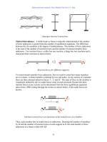
a true hinge. The joining members at a joint are often connected to each other through a
plate, called a gusset plate, either by bolts or by welding.
Five angle members connected by a gusset plate.
This kind of connection is closer to a rigid connection than to a hinged connection.
Nonetheless, we still assume the connection can be treated as a hinge as long as external
loads are applied at the joints only. This is because the triangular configuration of the
truss structure minimizes any moment action in the members and the predominant force

in each member is always the axial force. The stress in a truss member induced by the
rigid connection is called the secondary stress, which is negligible for most practical
cases. We shall examine the importance of secondary stress through an example.
Example 4. Find the end-moments of the two-bar truss shown, if all connections are
rigid. The section of both members are square with side dimension of 20 cm. E=1,000
kN/cm
2
. Discuss the significance of the secondary stress for three cases:
θ
=60
o
, 90
o
and
120
o
.
Two-bar truss example.
Solution. For the dimension given, EI=13,33.33 kN-m
2
, and EA=400,000 kN. If we treat
the structure as a rigid frame, we shall find member-end moments in addition to axial
force. If we treat the structure as a truss, we will have zero member-end moment and
only axial force in each member. We shall present the truss analysis results and the frame
analysis results in the table that follows. Because of symmetry, we need to concentrate on
one member only. It turns out that the end-moments at both ends of member ab are the
same. We need to examine the maximum compressive stress at node b only as a way of
evaluating the relative importance of secondary stress.
50 kN
4 m

a
c
b
θ
d
d
Other Topics by S. T. Mau
285
Truss and Frame Solutions
θ
=60
o
θ
=90
o
θ
=120
o
Member force/stress results
Truss Frame Truss Frame Truss Frame
Member compression(kN) 28.87 28.84 35.35 35.27 50.00 49.63
Moment at end b (kN-cm) 0 8.33 0 17.63 0 42.98
σ
due to axial force (kN/cm
2
)
0.072 0.072 0.088 0.088 0.125 0.124
σ
due to moment (kN/cm
2

)
0 0.006 0 0.013 0 0.032
Total σ (kN/cm
2
)
0.072 0.078 0.088 0.101 0.125 0.156
Error (truss result as base) 8.3% 15% 25%
In computing the normal stress from moment, we have used the formula:
σ
=
I
Mc
where c is the half height of the section. We observe that the compressive stress
computed from a rigid connection assumption is higher than that from the hinge
connection assumption. The error becomes larger when the angle
θ
becomes larger. The
results of the above analysis, however, are those for the worse possible case, because in
reality node a and node c would not have been fixed completely if the basic triangle a-b-c
is part of a larger truss configuration. Nonetheless, secondary stress should be considered
when the angle between two joining members becomes greater than 90
o
.
5.Composite Structures
We have learned the methods of analysis for truss structures and beam/frame structures.
In reality, many structures are composite structures in the sense that both truss and frame
members are used in a single structure. Bridge and building structures are often
composite structures as illustrated in the figure below, in which thin lines represent truss
members and thick lines represent frame members.
Cable-stay bridge and building frame as composite structure examples.

Other Topics by S. T. Mau
286
The analysis of composite structures can be accomplished with either the force method or
the displacement method. All computer packages allow the mixture of truss and frame
members. For very simple composite structures, hand calculation can be effective as
shown in the example below.
Example 5. As a much simplified model of a cable-stay bridge, the composite structure
shown is subjected to a single load at the center. Find the force in the cables. The cross-
sectional properties: A
cable
= 100 cm
2
, A
beam
= 180 cm
2
, and I
beam
=19,440 cm
4
. E=20,000
kN/cm
2
for both the cables and the beam. Neglect the axial deformation effect of the
beam.
Beam-Cable composite structure.
Because of symmetry, node b will have a downward deflection only, without a rotation.
We need to concentrate on only half of the structure. Denoting the downward deflection
as x, we observe that the elongation of the cable and the member rotation of member ab
are related to x.

∆
cable
=
5
3
x
φ
ab
=
4
1
x
Deflected configuration.
The vertical force equilibrium at node b involves the shear force of the beam, the vertical
component of the force in the cable and the externally applied load.
3 m
4 m
4 m
a
b
c
100 kN
4 m
3 m
b
a
x
φ
ab
5 m

Other Topics by S. T. Mau
287
F
cable
=
L
EA
∆
cable
=
L
EA
5
3
x =
500
0)(20000)(10
5
3
x =2400x
(F
cable
)
verticle
=
5
3
F
cable
=1440x

V
beam
= 12
L
EK
φ
ab
= 12
(400)(400)
440)(20000)(19
4
1
x =7290x
The equilibrium equation for vertical forces at node b calls for the sum of the shear force
in the beam and the vertical component of the cable force be equal to half of the
externally applied load, and the equation appears as:
1440x + 7290x = 50 x = 0.00573 cm
The shear force in the beam is
V
beam
=7290x=41.8 kN
The tension in the cables is
F
cable
=2400x= 13.8 kN.
6. Materials Non-linearity
We have assumed that materials are linearly elastic. This means that the stress-strain
relationship is proportional (linear)and when stress is removed, the strain will return to
the original state of zero strain (elastic). In general, however, a stress-strain relationship
can be elastic but nonlinear or inelastic and nonlinear. In truss and beam/frame analysis,

we deals with only uni-axial stress-strain relationship. The figure below illustrates
different uni-axial stress-strain relationships.
Other Topics by S. T. Mau
288
Various uni-axial stress-strain relationships.
The linear analysis we have been learning is valid only for linear material behavior, but,
as illustrated for the concrete stress-strain relationship, a linear relationship is a good
approximation if the stress-strain level is limited to a certain range. The highest level of
stress can be sustained by a material is called the ultimate strength, which is usually
beyond the linear region. Present design practice does require the consideration of the
ultimate strength, but the design process has been developed in such a way that a linear
analysis is still useful for preliminary design. Interested reader is encouraged to study
advanced strength of materials for nonlinear material behavior.
7. Geometric Non-linearity
A basic assumption in the linear structural analysis is that the deflected configuration is
very close to the original configuration. This is called the small-deflection assumption.
With this assumption, we can use the original configuration to set up equilibrium
equations. If, however, the deflection is not “small”, then the error induced by the small
deflection assumption could be too large to be ignored.
We will use the following example to illustrate the error of a small deflection assumption.
Example 6. For the two-bar truss shown, quantify the error of a small-deflection
analysis on the load-deflection relationship at node b. The two bars are identical and are
assumed to keep a constant cross-section area even under large strain.
ε
σ
ε
σ
ε
σ
ε

σ
E
lastic, linear
E
lastic, non-linear
E
lastic-plastic-hardening (steel)
N
onlinear, inelastic(concrete)
Other Topics by S. T. Mau
289
The last assumption about a constant cross-section area is to ignore the Poisson’s effect
and to simplify the analysis. We further assume the material remains linear-elastic so as
to isolate materials non-linearity effect from the geometric non-linearity effect we are
investigating herein
Two-bar truss example.
Solution. We shall derive the load-deflection relationship with and without the small-
deflection assumption.
Deflected configuration as the base of the equilibrium equation.
Denote the compression force in the two bars by F, we can write the vertical force
equilibrium equation at node b as
P=2F
vertical
The small-deflection assumption allows us to write
F
vertical
= F (
L
d
)

The bar shortening,
∆
,is geometrically related to the vertical deflection at b:
∆
=
δ
(
L
d
)
P
r
d
ac
b
r
P
r
d
ac
b
r
δ
L
L
’
Other Topics by S. T. Mau
290
The bar force is related to bar shortening by
F=

L
EA
∆
Combining the above equations, we obtain the load-deflection (P-
δ
) relationship
according to the small-deflection assumption:
P=2
L
EA
(
L
d
)
δ
(
L
d
)= 2EA(
L
d
)
3
(
d
δ
)(4)
For large deflection, we have to use the deflected configuration to compute bar
shortening and the vertical component of the bar force.
F

vertical
= F (
L'
-d
δ
)
∆
= L-L’
F=
L
EA
∆
= EA(1-
L
L'
)
P=2F
vertical
=2 EA(1-
L
L'
)(
L'
-d
δ
)(5)
We can express Eq. 5 in terms of two non-dimensional geometric factors, a/d and
δ
/d, as
shown below.

L’=
22
)(
δ
-da +
L=
22
da +
Dividing both sides by d, we have

d
L'
=
22
)1()(

δ
d
-
d
a
+
d
L
=
1 )(
2
+
d
a

Also,
L'
-d
δ
=
/dL'
d-
δ/
1
We can see that Eq. 4 and Eq. 5 depend on only the two geometric factors: the original
slope of the bar, a/d, and the deflection ratio,
δ
/d. Thus, the error of the small-deflection
assumption also depends on these two factors. We study two cases of a/d, and four cases
of
δ
/d and tabulate the results in the following table.
Other Topics by S. T. Mau
291
Error of Small-Deflection Assumption as a Function of a/d and δ/d
a/d=1.00
δ
/d 0.01 0.05 0.10 0.15
Eq. 2:
EA
P
2
=(1-
L

L'
)(
L'
-d
δ
)
0.0035 0.0169 0.0325 0.0466
Eq. 1:
EA
P
2
= (
L
d
)
3
(
d
δ
)
0.0035 0.0177 0.0354 0.0530
Eq. 1 / Eq. 2 1.00 1.05 1.09 1.14
Error (%): 1- (Eq. 1 / Eq. 2) 0% 5% 9% 14%
a/d=2.00
δ
/d 0.01 0.05 0.10 0.15
Eq. 2:
EA
P
2

=(1-
L
L'
)(
L'
-d
δ
)
0.0009 0.0042 0.0079 0.0110
Eq. 1:
EA
P
2
= (
L
d
)
3
(
d
δ
)
0.0009 0.0045 0.0089 0.0134
Eq. 1 / Eq. 2 1.00 1.07 1.13 1.22
Error (%): 1- (Eq. 1 / Eq. 2) 0% 7% 13% 22%
The results indicate that as deflection becomes increasingly larger (
δ
/d varies from 0.01
to 0.15), the small-deflection assumption introduces a larger and larger error. This error
is larger for shallower configuration (larger a/d ratio). The P/2EA values are plotted in

the following figure to illustrate the size of the error. We may conclude that the small-
deflection assumption is reasonable for
δ
/d less than 0.05.
Error of small-deflection assumption.
It is clear from the above figure that the load-deflection relationship is no longer linear
when deflection becomes larger.
P
/2EA
δ
/d
0.150.100.05
error
a/d=1.00
P
/2EA
δ
/d
0.150.100.05
error
a/d=2.00
0.0134
0.0530
Other Topics by S. T. Mau
292
8. Structural Stability
In truss or frame analysis, members are often subjected to compression. If the
compression force reaches a critical value, a member or the whole structure may deflect
in a completely different mode. This phenomenon is called buckling or structural
instability. The following figure illustrates two buckling configurations relative to the

non-buckling configurations.
Buckling configurations of a column and a frame.
Mathematically, the buckling configuration is an alternative solution to a non-buckling
solution to the governing equation. Since a linear equation has only one unique solution,
a buckling solution can be found only for a nonlinear equation. We shall explore where
the non-linearity comes from via the equation of a column with hinged ends and
subjected to an axial compression.
Non-buckling and buckling configurations as solutions to the beam equation.
The governing equation of beam flexure is
2
2
dx
vd
=
EI
M
δ δ
∆
δ δ
∆
∆
P
P
x
v
Other Topics by S. T. Mau
293
Because of the axial load and the lateral deflection, M= −Pv. Thus the governing
equation becomes
2

2
dx
vd
+
EI
Pv
= 0
This equation is linear if P is kept constant, but nonlinear if P is a variable as it is in the
present case. The solution to the above equation is
v = A Sin(
EI
P
x)
where A is any constant. This form of solution to the governing equation must also
satisfy the end conditions: v=0 at x=0 and x=L. The condition at x=0 is automatically
satisfied, but the condition at x=L leads to either
A=0
or
Sin(
EI
P
L)=0
The former is the non-buckling solution. The latter, with A≠0, is the buckling solution,
which exists only if
EI
P
L= n
π
, n=1, 2, 3…
The load levels at which a buckling solution exists are called the critical load:

P
cr
=
2
22
L
n
π
EI n=1, 2, 3…
The lowest critical load is the buckling load.
P
cr
=
2
2
L
π
EI
The above derivation is based on the small deflection assumption and the analysis is
called linear buckling analysis. If the small deflection assumption is removed, then a
nonlinear buckling analysis can be followed. The linear analysis can identify the critical
load at which buckling is to occur but cannot trace the load-lateral deflection relationship
Other Topics by S. T. Mau
294
on the post-buckling path. Only a nonlinear buckling analysis can produce the post-
buckling path. Interested readers are encouraged to study Structural Stability to learn
about a full spectrum of stability problems, elastic and inelastic, linear and nonlinear.
Linear and nonlinear buckling analyses results.
9. Dynamic Effects
In all the previous analyses, the load is assumed to be static. Which means a load is

applied slowly so that the resulting deflection of the structure also occurs slowly and the
velocity and acceleration of any point of the structure during the deflection process are
small enough to be neglected. How slow is slow? What if velocity and acceleration
cannot be neglected?
We know from Newton’s Second Law, or the derivative of it, that the product of a mass
and its acceleration constitutes an inertia term equivalent to force. In an equilibrium
system, this term, called D’Alembert force, can be treated as a negative force and all the
static equilibrium equations would apply. From physics, we learn that a moving subject
often encounters resistance either from within the subject or from the medium it is
moving through. This resistance, called damping, in its simplest form, can be represented
by the product of the velocity of the subject and a constant. Including both the inertia
term and the damping term in the equilibrium equations of a structure is necessary for
responses of a structure excited by wind, blast, earthquake excitations or any sudden
movement of the support or part of the structure. The dynamics effects are effects caused
by the presence of the inertia and the damping in a structural system and the associated
motion of the structure is called vibration. The equilibrium including dynamic effects is
called dynamic equilibrium.
It is not easy to quantify an excitation as a static one, but it is generally true that the
dynamic effects can be neglected if the excitation is gradual in the sense that it takes an
order longer to complete than the natural vibration period of the structure. The concept
of the natural vibration period can be easily illustrated by an example.
∆
P
∆
P
P
cr
P
ost-buckling path
L

inear analysis
P
re-buckling path