Fundamentals of Structural Analysis Episode 2 Part 7 pps

Other Topics by S. T. Mau
295
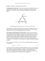
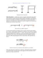
Example 7. Find the natural vibration period of a cantilever beam as shown. EI is
constant and the mass is uniformly distributed with a density
ρ
per unit length of the
beam. Assume there is no damping in the system.
A cantilever beam with uniformly distributed mass.
Solution. We shall limit ourselves to exploring the lateral vibration of the beam, although
the beam can also have vibration in the axial direction. A rigorous analysis would
consider the dynamic equilibrium of a typical element moving laterally. The resulting
governing equation would be a partial differential equation with two independent
variables, a spatial variable, x, and a time variable, t. The system would have infinite
degrees of freedom because the spatial variable, x, is continuous and represents an
infinite number of points along the beam. We shall pursue an approximate analysis by
lumping the total mass of the beam at the tip of the beam. This results in a single degree
of freedom (SDOF) system because we need to consider dynamic equilibrium only at the
tip.
Dynamic equilibrium of a distributed mass system and a lumped mass system.
The dynamic equilibrium of this SDOF system is shown in the above figure. The
dynamic equilibrium equation of the lumped mass is
m
2
2
dt
vd
+kv =0 (6)
where m=
ρ
L and k is the force per unit length of lateral deflection at the tip. We learn
from beam analysis that the force at the tip of the beam needed to produce a unit tip

deflection is 3EI/L
3
, thus k = 3EI/L
3
.
L
x
v(x)
ρ
dx
2
2
dt
vd
V
V+dV
L
v
m
2
2
dt
vd
kv
x
Other Topics by S. T. Mau
296
An equivalent form of Eq. 3 is
2
2

dt
vd
+
m
k
v =0 (6)
The factor associated with v in the above equation is a positive quantity and can be
replaced by
ω
2
=
m
k
(7)
Then Eq. 6 can be put in the following form:
2
2
dt
vd
+
ω
2
v =0 (6)
The general solution to Eq. 6 is
v = A Sin n
ω
t + B Cos n
ω
t, n=1, 2, 3… (5)
The constants A and B are to be determined by the position and velocity at t=0. No matter

what are the conditions, which are called initial conditions, the time variation of the
lateral deflection at the tip is sinusoidal or harmonic with a frequency of n
ω
. The lowest
frequency,
ω
, for n=1, is called the fundamental frequency of natural vibration. The other
frequencies are frequencies of higher harmonics. The motion, plotted against time, is
periodic with a period of T:
T=
ω
π
2
(6)
Harmonic motion with a period T.
In the present case, if EI=24,000 kN-m
2
, L=6 m and
ρ
=100 kg/m, then k = 3EI/L
3
=333.33
kN/m, m=
ρ
L= 600kg, and
ω
2
=k/m=0.555 (kN/m.kg)=555(1/sec
2
). The fundamental

v
t
T
Other Topics by S. T. Mau
297
vibration frequency is
ω
=23.57 rad/sec, and the fundamental vibration period is T=0.266
sec. The inverse of T , denoted by f, is called the circular frequency:
f =
T
1
(6)
which has the unit of circle per second (cps), which is often referred to as Hertz or Hz. In
the present example, the beam has a circular frequency of 3.75 cps or 3.75 Hz.
Interested readers are encouraged to study Structural Dynamics, in which undamped
vibration, damped vibration, free vibration and forced vibration of SDOF system, multi-
degree-of-freedom (MDOF) system and other interesting and useful subjects are
explored.
299
Matrix Algebra Review
1. What is a Matrix?
A matrix is a two-dimensional array of numbers or symbols that follows a set of
operating rules. A matrix having m rows and n columns is called a matrix of order m-by-n
and can be represented by a bold-faced letter with subscripts representing row and
column numbers, e.g., A
3x7
. If m=1 or n=1, then the matrix is called a row matrix or a
column matrix, respectively. If m=n, then the matrix is called a square matrix. If m=n=1,
then the matrix is degenerated into a scalar.

Each entry of the two dimensional array is called an element, which is often represented
by a plain letter or a lower case letter with subscripts representing the locations of the row
and column in the matrix. For example a
23
is the element in matrix A located at the
second row and third column. Diagonal elements of a square matrix A can be represented
by a
ii
. A matrix with all elements equal to zero is called a null matrix. A square matrix
with all non-diagonal elements equal to zero is called a diagonal matrix. A diagonal
matrix with all the diagonal elements equal to one is called a unit or identity matrix and is
represented by I. A square matrix whose elements satisfy a
ij
=a
ji
is called a symmetric
matrix. An identity matrix is also a symmetric matrix. A transpose of a matrix is another
matrix with all the row and column elements interchanged: (a
T
)
ij
=a
ji
. The order of a
transpose of an m-by-n matrix is n-by-m. A symmetric matrix is one whose transpose is
the same as the original matrix: A
T

=

A. A skew matrix is a square matrix satisfying a
ij
=
−a
ji
. The diagonal elements of a skew matrix are zero.
Exercise 1. Fill in the blanks in the sentences below.
A=
⎥
⎥
⎥
⎦
⎤
⎢
⎢
⎢
⎣
⎡
101
37
42
B=
⎥
⎦
⎤
⎢
⎣
⎡
1034
172

C=
⎥
⎥
⎥
⎦
⎤
⎢
⎢
⎢
⎣
⎡
843
451
312
D=
⎪
⎭
⎪
⎬
⎫
⎪
⎩
⎪
⎨
⎧
7
5
2
E=
[

]
752
F=
⎥
⎥
⎥
⎦
⎤
⎢
⎢
⎢
⎣
⎡
800
050
002
G=
⎥
⎥
⎥
⎦
⎤
⎢
⎢
⎢
⎣
⎡
100
010
001

H=
⎥
⎥
⎥
⎦
⎤
⎢
⎢
⎢
⎣
⎡
000
000
000
K=
⎥
⎥
⎥
⎦
⎤
⎢
⎢
⎢
⎣
⎡
−−
−
043
401
310

Matrix A is a ___-by___ matrix and matrix B is a ___-by___ matrix.
Matrix A is the _____________ of matrix B and vice versa.
Matrix Algebra Review by S. T. Mau
300
Matrices C and F are _________ matrices with ________ rows and ________ columns.
Matrix D is a ________ matrix and matrix E is a ______ matrix; E is the __________ of
D.
Matrix G is an ________ matrix; matrix H is a ______ matrix; matrix K is a _______
matrix.
In the above, there are _____ symmetric matrices and they are __________________.
2. Matrix Operating Rules
Only matrices of the same order can be added to or subtracted from each other. The
resulting matrix is of the same order with an element-to-element addition or subtraction
from the original matrices.
C+F =
⎥
⎥
⎥
⎦
⎤
⎢
⎢
⎢
⎣
⎡
843
451
312
+
⎥

⎥
⎥
⎦
⎤
⎢
⎢
⎢
⎣
⎡
800
050
002
=
⎥
⎥
⎥
⎦
⎤
⎢
⎢
⎢
⎣
⎡
1643
4101
314
C−F =
⎥
⎥
⎥

⎦
⎤
⎢
⎢
⎢
⎣
⎡
843
451
312
−
⎥
⎥
⎥
⎦
⎤
⎢
⎢
⎢
⎣
⎡
800
050
002
=
⎥
⎥
⎥
⎦
⎤

⎢
⎢
⎢
⎣
⎡
043
401
310
The following operations using matrices defined in the above are not admissible: A+B,
B+C, D−E, and D−G.
Multiplication of a matrix by a scalar results in a matrix of the same order with each
element multiplied by the scalar. Multiplication of a matrix by another matrix is
permissible only if the column number of the first matrix matches with the row number
of the second matrix and the resulting matrix has the same row number as the first matrix
and the same column number as the second matrix. In symbols, we can write
B x D = Q and Q
ij
=
∑
=
3
1k
kjik
DB
Using the numbers given above we have
Q =B x D = BD =
⎥
⎦
⎤
⎢

⎣
⎡
1034
172
⎪
⎭
⎪
⎬
⎫
⎪
⎩
⎪
⎨
⎧
7
5
2
=
⎭
⎬
⎫
⎩
⎨
⎧
++
++
x701 3x5x24
1x7 7x5x22
=
⎭

⎬
⎫
⎩
⎨
⎧
113
46
Matrix Algebra Review by S. T. Mau
301
P =Q x E = QE =
⎭
⎬
⎫
⎩
⎨
⎧
113
46
[
]
752
=
⎥
⎦
⎤
⎢
⎣
⎡
791565226
32223092

We can verify numerically that
P =QE = BDE= (BD)E= B(DE)
We can also verify multiplying any matrix by an identity matrix of the right order will
result in the same original matrix, thus the name identity matrix.
The transpose operation can be used in combination with multiplication in the following
way, which can be easily derived from the definition of the two operations.
(AB)
T
=B
T
A
T
and (ABC)
T
=C
T
B
T
A
T
Exercise 2. Complete the following operations.
E B =
⎥
⎦
⎤
⎢
⎣
⎡
63
25

⎥
⎦
⎤
⎢
⎣
⎡
1034
172
=
DE =
⎪
⎭
⎪
⎬
⎫
⎪
⎩
⎪
⎨
⎧
7
5
2
[
]
752
=
3. Matrix Inversion and Solving Simultaneous Algebraic
Equations

A square matrix has a characteristic value called determinant. The mathematical
definition of a determinant is difficult to express in symbols, but we can easily learn the
way of computing the determinant of a matrix by the following examples. We shall use
Det to represent the value of a determinant. For example, DetA means the determinant of
matrix A.
Det [5]=5
Det
⎥
⎦
⎤
⎢
⎣
⎡
63
25
= 5x Det [6] −3x Det [2] = 30 – 6 =24
Det
⎥
⎥
⎥
⎦
⎤
⎢
⎢
⎢
⎣
⎡
963
852
741

= 1x Det
⎥
⎦
⎤
⎢
⎣
⎡
96
85
−2x Det
⎥
⎦
⎤
⎢
⎣
⎡
96
74
+ 3x Det
⎥
⎦
⎤
⎢
⎣
⎡
85
74
Matrix Algebra Review by S. T. Mau
302
=1x(−3)−2x(−6)+3x(−3)=0

A matrix with a zero determinant is called a singular matrix. A non-singular matrix A
has an inverse matrix A
-1
, which is defined by
AA
-1
=I
We can verify that the two symmetric matrices at the left-hand-side (LHS) of the
following equation are inverse to each other.
⎥
⎥
⎥
⎦
⎤
⎢
⎢
⎢
⎣
⎡
−
−
812
141
211
⎥
⎥
⎥
⎦
⎤
⎢

⎢
⎢
⎣
⎡
−
−
−−
113
13/43/10
33/103/31
=
⎥
⎥
⎥
⎦
⎤
⎢
⎢
⎢
⎣
⎡
100
010
001
⎥
⎥
⎥
⎦
⎤
⎢

⎢
⎢
⎣
⎡
−
−
−−
113
13/43/10
33/103/31
⎥
⎥
⎥
⎦
⎤
⎢
⎢
⎢
⎣
⎡
−
−
812
141
211
=
⎥
⎥
⎥
⎦

⎤
⎢
⎢
⎢
⎣
⎡
100
010
001
This is because the transpose of an identity matrix is also an identity matrix and
(AB)=I (AB)
T
=(B
T
A
T
)=(BA)=I
T
=I
The above statement is true only for symmetric matrices.
There are different algorithms for finding the inverse of a matrix. We shall introduce one
that is directly linked to the solution of simultaneous equations. In fact, we shall see
matrix inversion is an operation more involved than solving simultaneous equations.
Thus, if solving simultaneous equation is our goal, we need not go through a matrix
inversion first.
Consider the following simultaneous equations for three unknowns.
x
1
+ x
2

+ 2x
3
= 1
x
1
+ 4x
2
− x
3
= 0
2x
1
− x
2
+ 8x
3
= 0
The matrix representation of the above is
⎥
⎥
⎥
⎦
⎤
⎢
⎢
⎢
⎣
⎡
−
−

812
141
211
⎪
⎭
⎪
⎬
⎫
⎪
⎩
⎪
⎨
⎧
3
2
1
x
x
x
=
⎪
⎭
⎪
⎬
⎫
⎪
⎩
⎪
⎨
⎧

0
0
1
Matrix Algebra Review by S. T. Mau
303
Imagine we have two additional sets of problems with three unknowns and the same
coefficients in the LHS matrix but different right-hand-side (RHS) figures.
⎥
⎥
⎥
⎦
⎤
⎢
⎢
⎢
⎣
⎡
−
−
812
141
211
⎪
⎭
⎪
⎬
⎫
⎪
⎩
⎪

⎨
⎧
3
2
1
x
x
x
=
⎪
⎭
⎪
⎬
⎫
⎪
⎩
⎪
⎨
⎧
0
1
0
and
⎥
⎥
⎥
⎦
⎤
⎢
⎢

⎢
⎣
⎡
−
−
812
141
211
⎪
⎭
⎪
⎬
⎫
⎪
⎩
⎪
⎨
⎧
3
2
1
x
x
x
=
⎪
⎭
⎪
⎬
⎫

⎪
⎩
⎪
⎨
⎧
1
0
0
Since the solutions for the three problems are different, we should use different symbols
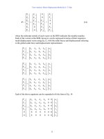
for them. But, we can put all three problems in one single matrix equation below.
⎥
⎥
⎥
⎦
⎤
⎢
⎢
⎢
⎣
⎡
−
−
812
141
211
⎥
⎥
⎥
⎦
⎤

⎢
⎢
⎢
⎣
⎡
333231
232221
131211
xxx
xxx
xxx
=
⎥
⎥
⎥
⎦
⎤
⎢
⎢
⎢
⎣
⎡
100
010
001
Or,
AX= I
By definition, X is the inverse of A. The first column of X contains the solution to the
first problem, and the second column contains the solution to the second problem, etc.
To find X, we shall use a process called Gaussian Elimination, which has several

variations. We shall present two variations. The Gaussian process uses each equation
(row in the matrix equation) to combine with another equation in a linear way to reduce
the equations to a form from which a solution can be obtained.
(1) The first version. We shall begin by a forward elimination process, followed by a
backward substitution process. The changes as the result of each elimination/substitution
are reflected in the new content of the matrix equation.
Forward Elimination. Row 1 is multiplied by (–1) and added to row 2 to replace row 2,
and row 1 is multiplied by (−2) and added to row 3 to replace row 3, resulting in:
⎥
⎥
⎥
⎦
⎤
⎢
⎢
⎢
⎣
⎡
−
−
430
330
211
⎥
⎥
⎥
⎦
⎤
⎢
⎢

⎢
⎣
⎡
333231
232221
131211
xxx
xxx
xxx
=
⎥
⎥
⎥
⎦
⎤
⎢
⎢
⎢
⎣
⎡
−
−
102
011
001
Row 2 is added to row 3 to replace row 3, resulting in:
⎥
⎥
⎥
⎦

⎤
⎢
⎢
⎢
⎣
⎡
−
100
330
211
⎥
⎥
⎥
⎦
⎤
⎢
⎢
⎢
⎣
⎡
333231
232221
131211
xxx
xxx
xxx
=
⎥
⎥
⎥

⎦
⎤
⎢
⎢
⎢
⎣
⎡
−
−
113
011
001
Matrix Algebra Review by S. T. Mau
304
The forward elimination is completed and all elements below the diagonal line in A are
zero.
Backward Substitution. Row 3 is multiplied by (3) and added to row 2 to replace row 2,
and row 3 is multiplied by (−2) and added to row 1 to replace row 1, resulting in:
⎥
⎥
⎥
⎦
⎤
⎢
⎢
⎢
⎣
⎡
100
030

011
⎥
⎥
⎥
⎦
⎤
⎢
⎢
⎢
⎣
⎡
333231
232221
131211
xxx
xxx
xxx
=
⎥
⎥
⎥
⎦
⎤
⎢
⎢
⎢
⎣
⎡
−
−

−−
113
3410
227
Row 2 is multiplied by (−1/3) and added to row 1 to replace row 1, resulting in:
⎥
⎥
⎥
⎦
⎤
⎢
⎢
⎢
⎣
⎡
100
030
001
⎥
⎥
⎥
⎦
⎤
⎢
⎢
⎢
⎣
⎡
333231
232221

131211
xxx
xxx
xxx
=
⎥
⎥
⎥
⎦
⎤
⎢
⎢
⎢
⎣
⎡
−
−
−−
113
3410
33/103/31
Normalization. Now that matrix A is reduced to a diagonal matrix, we further reduce it
to an identity matrix by dividing each row by the diagonal element of each row, resulting
in:
⎥
⎥
⎥
⎦
⎤
⎢

⎢
⎢
⎣
⎡
100
010
001
⎥
⎥
⎥
⎦
⎤
⎢
⎢
⎢
⎣
⎡
333231
232221
131211
xxx
xxx
xxx
=
⎥
⎥
⎥
⎦
⎤
⎢

⎢
⎢
⎣
⎡
−
−
−−
113
13/43/10
33/103/31
Or,
X=
⎥
⎥
⎥
⎦
⎤
⎢
⎢
⎢
⎣
⎡
333231
232221
131211
xxx
xxx
xxx
=
⎥

⎥
⎥
⎦
⎤
⎢
⎢
⎢
⎣
⎡
−
−
−−
113
13/43/10
33/103/31
Note that X is also symmetric. It can be derived that the inverse of a symmetric matrix is
also symmetric.
(2) The second version. We combine the forward and backward operations and the
normalization together to reduce all off-diagonal terms to zero, one column at a time. We
reproduce the original matrix equation below.
⎥
⎥
⎥
⎦
⎤
⎢
⎢
⎢
⎣
⎡

−
−
812
141
211
⎥
⎥
⎥
⎦
⎤
⎢
⎢
⎢
⎣
⎡
333231
232221
131211
xxx
xxx
xxx
=
⎥
⎥
⎥
⎦
⎤
⎢
⎢
⎢

⎣
⎡
100
010
001
Matrix Algebra Review by S. T. Mau
305
Starting with the first row, we normalize the diagonal element of the first row to one (in
this case, it is already one) by dividing the first row by the vale of the diagonal element.
Then we use the new first row to eliminate the first column elements in row 2 and row 3,
resulting in
⎥
⎥
⎥
⎦
⎤
⎢
⎢
⎢
⎣
⎡
−
−
430
330
211
⎥
⎥
⎥
⎦

⎤
⎢
⎢
⎢
⎣
⎡
333231
232221
131211
xxx
xxx
xxx
=
⎥
⎥
⎥
⎦
⎤
⎢
⎢
⎢
⎣
⎡
−
−
102
011
001
We repeat the same operation with the second row and the diagonal element of the
second row to eliminate the second column elements in row 1 and row 3, resulting in

⎥
⎥
⎥
⎦
⎤
⎢
⎢
⎢
⎣
⎡
−
100
110
301
⎥
⎥
⎥
⎦
⎤
⎢
⎢
⎢
⎣
⎡
333231
232221
131211
xxx
xxx
xxx

=
⎥
⎥
⎥
⎦
⎤
⎢
⎢
⎢
⎣
⎡
−
−
−
113
03/13/1
03/13/4
The same process is done using the third row and the diagonal element of the third row,
resulting in
⎥
⎥
⎥
⎦
⎤
⎢
⎢
⎢
⎣
⎡
100

010
001
⎥
⎥
⎥
⎦
⎤
⎢
⎢
⎢
⎣
⎡
333231
232221
131211
xxx
xxx
xxx
=
⎥
⎥
⎥
⎦
⎤
⎢
⎢
⎢
⎣
⎡
−

−
−−
113
13/43/10
33/103/31
Or,
X=
⎥
⎥
⎥
⎦
⎤
⎢
⎢
⎢
⎣
⎡
333231
232221
131211
xxx
xxx
xxx
=
⎥
⎥
⎥
⎦
⎤
⎢

⎢
⎢
⎣
⎡
−
−
−−
113
13/43/10
33/103/31
The same process can be used to find the solution for any given column on the RHS,
without finding the inverse first. This is left to readers as an exercise.
Exercise 3. Solve the following problem by the Gaussian Elimination method.
⎥
⎥
⎥
⎦
⎤
⎢
⎢
⎢
⎣
⎡
−
−
812
141
211
⎪
⎭

⎪
⎬
⎫
⎪
⎩
⎪
⎨
⎧
3
2
1
x
x
x
=
⎪
⎭
⎪
⎬
⎫
⎪
⎩
⎪
⎨
⎧
1
6
3
Forward Elimination. Row 1 is multiplied by (–1) and added to row 2 to replace row 2,
and row 1 is multiplied by (−2) and added to row 3 to replace row 3, resulting in:

Matrix Algebra Review by S. T. Mau
306
⎥
⎥
⎥
⎦
⎤
⎢
⎢
⎢
⎣
⎡
−
−
430
330
211
⎪
⎭
⎪
⎬
⎫
⎪
⎩
⎪
⎨
⎧
3
2
1

x
x
x
=
⎪
⎭
⎪
⎬
⎫
⎪
⎩
⎪
⎨
⎧
Row 2 is added to row 3 to replace row 3, resulting in:
⎥
⎥
⎥
⎦
⎤
⎢
⎢
⎢
⎣
⎡
−
100
330
211
⎪

⎭
⎪
⎬
⎫
⎪
⎩
⎪
⎨
⎧
3
2
1
x
x
x
=
⎪
⎭
⎪
⎬
⎫
⎪
⎩
⎪
⎨
⎧
Backward Substitution. Row 3 is multiplied by (3) and added to row 2 to replace row 2,
and row 3 is multiplied by (−2) and added to row 1 to replace row 1, resulting in:
⎥
⎥

⎥
⎦
⎤
⎢
⎢
⎢
⎣
⎡
100
030
011
⎪
⎭
⎪
⎬
⎫
⎪
⎩
⎪
⎨
⎧
3
2
1
x
x
x
=
⎪
⎭

⎪
⎬
⎫
⎪
⎩
⎪
⎨
⎧
Row 2 is multiplied by (−1/3) and added to row 1 to replace row 1, resulting in:
⎥
⎥
⎥
⎦
⎤
⎢
⎢
⎢
⎣
⎡
100
030
001
⎪
⎭
⎪
⎬
⎫
⎪
⎩
⎪

⎨
⎧
3
2
1
x
x
x
=
⎪
⎭
⎪
⎬
⎫
⎪
⎩
⎪
⎨
⎧
Normalization. Now that matrix A is reduced to a diagonal matrix, we further reduce it
to an identity matrix by dividing each row by the diagonal element of each row, resulting
in:
⎥
⎥
⎥
⎦
⎤
⎢
⎢
⎢

⎣
⎡
100
010
001
⎪
⎭
⎪
⎬
⎫
⎪
⎩
⎪
⎨
⎧
3
2
1
x
x
x
=
⎪
⎭
⎪
⎬
⎫
⎪
⎩
⎪

⎨
⎧
If, however, the inverse is already obtained, then the solution for any given column on the
RHS can be obtained by a simple matrix multiplication as shown below.
AX=Y
Multiply both sides with A
-1
, resulting in
A
-1
AX= A
-1
Y
Or,
Matrix Algebra Review by S. T. Mau
307
X= A
-1
Y
This process is left as an exercise.
Exercise 4. Solve the following equation by using the inverse matrix of A.
⎥
⎥
⎥
⎦
⎤
⎢
⎢
⎢
⎣

⎡
−
−
812
141
211
⎪
⎭
⎪
⎬
⎫
⎪
⎩
⎪
⎨
⎧
3
2
1
x
x
x
=
⎪
⎭
⎪
⎬
⎫
⎪
⎩

⎪
⎨
⎧
1
6
3
A=
⎥
⎥
⎥
⎦
⎤
⎢
⎢
⎢
⎣
⎡
−
−
812
141
211
A
-1
=
⎥
⎥
⎥
⎦
⎤

⎢
⎢
⎢
⎣
⎡
−
−
−−
113
13/43/10
33/103/31
⎪
⎭
⎪
⎬
⎫
⎪
⎩
⎪
⎨
⎧
3
2
1
x
x
x
== A
-1
⎪

⎭
⎪
⎬
⎫
⎪
⎩
⎪
⎨
⎧
−
−
2
1
8
=
⎥
⎥
⎥
⎦
⎤
⎢
⎢
⎢
⎣
⎡
−
−
−−
113
13/43/10

33/103/31
⎪
⎭
⎪
⎬
⎫
⎪
⎩
⎪
⎨
⎧
1
6
3
=
⎪
⎭
⎪
⎬
⎫
⎪
⎩
⎪
⎨
⎧
Problem. Solve the following equation by (1) Gaussian elimination, and (2) matrix
inversion, using the known inverse of the matrix at the LHS.
⎥
⎥
⎥

⎦
⎤
⎢
⎢
⎢
⎣
⎡
−
−
−−
113
13/43/10
33/103/31
⎪
⎭
⎪
⎬
⎫
⎪
⎩
⎪
⎨
⎧
3
2
1
x
x
x
=

⎪
⎭
⎪
⎬
⎫
⎪
⎩
⎪
⎨
⎧
1
6
3
Matrix Algebra Review by S. T. Mau
308
309309
Solution to Problems
02 Truss Analysis: Matrix Displacement Method
Problem 1: k
33
= EAC
2
/L

= 7.2 MN/m, k
34
= EACS/L

= 9.6 MN/m, k
31

= − EAC
2
/L

= −7.2
MN/m. The effect of the change of the numbering is only in the location at which each
quantity is to appear but not in its value.
Problem 2. The change of numbering for members results in a switch between (k
G
)
2
and
(k
G
)
3
, but has no effect on the resulting stiffness equation, because the nodal
displacements are still the same. The constrained stiffness equation is identical to Eq. 16.
Problem 3.
Case (a): Member Solutions
Member
Force
(MN)
Elongation
(m)
Member
Force
(MN)
Elongation
(m)

1 0.375 0.011 8 0 0
2 0.375 0.011 9 0.625 0.031
3 0.375 0.011 10 0 0
4 0.375 0.011 11 -0.625 -0.031
5 -0.625 -0.031 12 -0.750 -0.023
6 0 0 13 -0.750 -0.023
7 0.625 -0.031
Case (a): Nodal Solutions
Node u(m) v(m) Node u(m) v(m)
1 0.000 0.000 5 0.045 0.00
2 0.011 -0.073 6 0.045 -0.073
3 0.023 -0.129 7 0.023 -0.129
4 0.034 -0.073 8 0.000 -0.073
The reactions are: 0.5 MN upward at both node 1 and node 5.
1
2
3
4
5
6
7
8
12
1
3
1
4
1
56
7

89
1
10
11
12
13
x
y
Solution to Problems by S. T. Mau
310310
Case (b): Member Solutions
Member
Force
(MN)
Elongation
(m)
Member
Force
(MN)
Elongation
(m)
1 0.563 0.017 8 0 0
2 0.563 0.017 9 0.312 0.016
3 0.187 0.006 10 0 0
4 0.187 0.006 11 -0.312 -0.016
5 -0.938 -0.041 12 -0.375 -0.011
6 1.000 0.040 13 -0.375 -0.011
7 -0.312 -0.016
Case (b): Nodal Solutions
Node u(m) v(m) Node u(m) v(m)

1 0.000 0.000 5 0.045 0.00
2 0.017 -0.128 6 0.039 -0.088
3 0.034 -0.073 7 0.028 -0.073
4 0.039 -0.041 8 0.017 -0.041
The reactions are: 0.75 MN upward at node 1 and 0.25 MN upward at node 5.
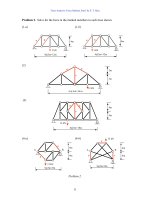
Problem 4: Discuss the kinematic stability of each of the plane truss shown.
(1) Stable, (2) Unstable, (3) Stable, (4) Unstable, (5) Stable, (6) Unstable, (7) Stable, (8)
Unstable, (9) Stable, (10) unstable.
03 Truss Analysis: Force Method, Part I
Problem 1.
(1-a)(1-b)(1-c)
1
2
3
4
5
6
7
8
12
1
3
1
4
1
56
7
89
1
10

11
12
13
x
y
3 kN
3 kN
4 kN
4 kN
−4 kN
5 kN
0 kN
8 kN
4 kN4 kN
8 kN
−5 kN
−5 kN
3 kN
3 kN
8 kN
3 kN
2 kN 6 kN
3 kN
3 kN
8 kN
−2.5 kN
4.5 kN 4.5 kN
−7.5 kN
0 kN
Solution to Problems by S. T. Mau

311311
(2-a)(2-b)(2-c)
(3-a)(3-b)(3-c)
(4-a)(4-b)(4-c)
Problem 2.
(1-a) F
a
= −0.625 kN, F
b
= −0.625 kN. (1-b) F
a
= −0.9375 kN, F
b
= 0.3125 kN.
(2) F
a
= −5.37 kN, F
b
= −5.37 kN, F
c
= −(F
a
)
y
− (F
b
)
y
= 4.80 kN
(3) F

a
= 2.5 kN, F
b
= −2.5 kN, F
c
= 0
(4-a) F
a
=0, F
b
=12.5 kN. (4-b) F
a
=0, F
b
=0, F
c
= −10 kN.
Problem 3.
(1)
⎥
⎥
⎥
⎥
⎥
⎥
⎥
⎦
⎤
⎢
⎢

⎢
⎢
⎢
⎢
⎢
⎣
⎡
−−
−
−−
−−−
0.1000.08.00
0.0000.16.00
00008.08.0
00006.06.0
00.10.00.008.0
00.00.10.106.0
⎪
⎪
⎪
⎭
⎪
⎪
⎪
⎬
⎫
⎪
⎪
⎪
⎩

⎪
⎪
⎪
⎨
⎧
6
5
4
3
2
1
F
F
F
F
F
F
=
⎪
⎪
⎪
⎭
⎪
⎪
⎪
⎬
⎫
⎪
⎪
⎪

⎩
⎪
⎪
⎪
⎨
⎧
−
0
5.0
0.1
0
0
0
(2)
⎥
⎥
⎥
⎥
⎥
⎥
⎥
⎦
⎤
⎢
⎢
⎢
⎢
⎢
⎢
⎢

⎣
⎡
−−
−
−
−
−−−
0.10.0008.00
0.00.1006.00
00008.08.0
00006.06.0
000.00.008.0
000.10.106.0
⎪
⎪
⎪
⎭
⎪
⎪
⎪
⎬
⎫
⎪
⎪
⎪
⎩
⎪
⎪
⎪
⎨

⎧
6
5
4
3
2
1
F
F
F
F
F
F
=
⎪
⎪
⎪
⎭
⎪
⎪
⎪
⎬
⎫
⎪
⎪
⎪
⎩
⎪
⎪
⎪

⎨
⎧
−
0
0
0.1
5.0
0
0
4 kN
4 kN
3 kN
3 kN
0 kN
0 kN
5 kN
3 kN
−3 kN
−5 kN
3 kN
3 kN
4 kN
3 kN3 kN
−5 kN
5 kN
−5 kN
−6 kN
−6 kN
4 kN
5 kN

5 kN
1.8 kN 3.2 kN
2.4 kN
−4 kN−3 kN
4 kN
1.12 kN
2.88 kN
−4.8 kN −1.4 kN
5 kN
0.84 kN3.84
2.4
4kN
5kN
4.32 kN
4.68 kN
−5.4 kN
−7.8 kN
6.24
3.24 3.24
5
5
2 kN
1 kN
0.5 kN 0.5 kN
1 kN 1 kN
0.5 kN 1.5 kN
−1.12 kN −1.12
0 kN
2 kN
2.24

−1 kN
0 kN
2.24
0 kN
1 kN
1.12
2.24
−1.12
−1 kN
1 kN
1 kN
1
4 kN
2 kN
1 kN
Solution to Problems by S. T. Mau
312312
Problem 4.
(1)
⎥
⎥
⎥
⎥
⎥
⎥
⎥
⎦
⎤
⎢
⎢

⎢
⎢
⎢
⎢
⎢
⎣
⎡
−−
−−−
−−−
−
−
0.10.05.067.00.00.0
0.00.05.067.00.10.0
0.00.10.00.10.00.1
0.00.138.05.00.00.0
0.00.063.0
83.00.00.0
0.00.063.083.00.00.0
⎪
⎪
⎪
⎭
⎪
⎪
⎪
⎬
⎫
⎪
⎪

⎪
⎩
⎪
⎪
⎪
⎨
⎧
−
0
5.0
0.1
0
0
0
=
⎪
⎪
⎪
⎭
⎪
⎪
⎪
⎬
⎫
⎪
⎪
⎪
⎩
⎪
⎪

⎪
⎨
⎧
−
−
−
5.0
5.0
5.0
88.0
63.0
63.0
(2)
⎥
⎥
⎥
⎥
⎥
⎥
⎥
⎦
⎤
⎢
⎢
⎢
⎢
⎢
⎢
⎢
⎣

⎡
−−
−−−
−−−
−
−
0.10.05.067.00.00.0
0.00.05.067.00.10.0
0.00.10.00.10.00.1
0.00.138.05.00.00.0
0.00.063.0
83.00.00.0
0.00.063.083.00.00.0
⎪
⎪
⎪
⎭
⎪
⎪
⎪
⎬
⎫
⎪
⎪
⎪
⎩
⎪
⎪
⎪
⎨

⎧
−
0
0.1
0.1
5.0
0
0
=
⎪
⎪
⎪
⎭
⎪
⎪
⎪
⎬
⎫
⎪
⎪
⎪
⎩
⎪
⎪
⎪
⎨
⎧
−
−
−

83.0
17.0
5.1
62.1
04.1
21.0
04 Truss Analysis: Force Method, Part II
Problem 5.
(1) 0.0526 mm to the right.
(2) There is no horizontal displacement at node 2.
(3) Node 5 moves to the right by 0.67 mm.
Problem 6.
(1) The force in member 10 is 8.86/0.172=51.51 kN.
(2) The force in member 6 is 1.62/0.174=9.31 kN.
05 Beam and Frame Analysis: Force Method, Part I
Problem 1.
(1)Determinate. (2) Determinate. (3) Indeterminate to the 1
st
degree. (4) Indeterminate to
the 2
nd
degree. (5)Indeterminate to the 3
rd
degree. (6) Indeterminate to the 4th degree. (7)
Indeterminate to the 15th degree. (8) Indeterminate to the 18th degree.
Solution to Problems by S. T. Mau
313313
Problem 2.
(1) (2)
(3) (4)

(5) (6)
(7) (8)
(9) (10)
10 kN
-50 kN-m
V
M
3.75 kN
18.75 kN-m
V
M
-6.25 kN
15 kN
-37.5 kN-m
V
M
10.31 kN
14.07 kN-m
V
M
-4.69 kN
3.4 m
17.52 kN-m
0 kN
-10 kN-m
V
M
1.25 kN
6.25 kN-m
V

M
-3.75 kN-m
-2.5 kN
10 kN-m
V
M
-12 kN
V
M
-36 kN-m
-15 kN-m
10 kN
-10 kN
10 kN
20 kN-m
20 kN-m
-20 kN-m
V
M
-2 kN
-4 kN
4 kN-m
2 kN-m
-4 kN-m
V
M
4 kN
4 kN
-4 kN-m
Solution to Problems by S. T. Mau

314314
(11)
(12)
(13)
(14)
T
10 kN
V
10 kN
M
50 kN-m
-10 kN
T
V
M
-2 kN
2 kN
10 kN-m
T
T
V
V
M
M
10 kN
-10 kN
-2 kN 2 kN
10 kN
-10 kN
2 kN

50 kN-m
10 kN-m
Solution to Problems by S. T. Mau
315315
(15)
(16)
06 Beam and Frame Analysis: Force Method, Part II
Problem 3.
(1)
Shear(Rotation) diagram(LEFT) and Moment(Deflection) digram (RIGHT).
(2)
Shear(Rotation) diagram(LEFT) and Moment(Deflection) digram (RIGHT).
(3)
Shear(Rotation) diagram(LEFT) and Moment(Deflection) digram (RIGHT).
T
T
V
V
M
M
2 kN
-2 kN
10 kN
2 kN
-50 kN-m
10 kN-m
L

/2EI
L

2

/8EI
0.064L
2

/EI
L
/3EI
-L/6EI
0.58L
-L
2

/8EI
-5L
3

/48EI
-L
3

/24EI