Gear Noise and Vibration Episode 1 Part 5 docx

Prediction
of
Dynamic
Effects
5.1. Modelling
of
gears
in 2-D
Static
determination
of
T.E. under load
is
sufficient
for
most drives
where
the
loading
is
relatively heavy
and the
inertias
are low so
that there
is
little
danger
of the
length

of
line
of
contact varying greatly
or of the
teeth
losing contact.
The
T.E.
is
then
the
input vibration and,
as the
system
remains reasonably linear
in its
behaviour,
it can be
modelled using
a
conventional
matrix approach
in the frequency
domain. Drives which
are
lightly
loaded
or
which drive high inertias, such

as
printing rolls,
may
lose
contact
with rather dramatic results.
It is
then possible
for the
teeth
to be in
contact
for
less than
10%
of the
time with rather large impulsive
forces
while
they
are in
contact.
The
simple assumption
of a
linear system with
an
input
displacement
of the

quasi-static T.E.
is
then
no
longer realistic
and a
more
detailed
model
is
required (see section
5.2 and
Chapter
11).
Even
when
the
teeth
do not
come
fully
out of
contact
the
simple
assumption
of a
linear system
can be
wildly unrealistic. This

is due to the
large variations
in the
true length
of the
contact line, partly
due to the
gear
flank
shapes
and
partly
due to the
vibration.
If the
nominal mean
elastic
deflection
in the
mesh
is of the
order
of 10
urn,
then
a
vibration
of 2
ujn
can

easily
alter
the
contact
stiffness
by a
factor
of 2 by
changing
the
length
of the
line
of
contact during
the
vibration.
A
simple assumption that
stiffness
is
proportional
to
nominal length
of
line
of
contact
is
near

the
truth
for
well-
aligned
spur gears
but not
true
for
misaligned
gears,
especially helicals.
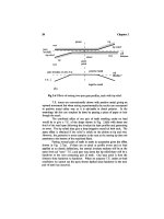
The
simplest realistic model
of a
pair
of
gears
is
shown
in
Fig.
5.1.
Axial
movements
are
negligible
or
ignored although
the

gears
are
taken
to be
helical. There
is
considerable simplification
if we
take
the
linear axis along
the
line
of
thrust
and
ignore
any
motion perpendicular
as
being small since
it
is
only
due to
(small)
friction
effects
which
are in the

main self-cancelling
for
helicals.
Four degrees
of freedom are
involved,
two
linear
and two
torsional
and
if the
system
is
linear with
a
constant contact
stiffness
Sc
the
estimation
of
response
is
simple.
A
force
P at the
contact will give linear
and

torsional responses
to
each
of the two
gears.
The
relative movement
d at P is the sum of the
four
responses together with
the
contact deflection
due to the
contact
stiffness
s
c
and
damping
coefficient
b
c
.
61
62
Chapter
5
pinion
yp
be

wheel
Fig 5.1
Simple
2-dimensional
model
of a
gear pair vibration.
It
is
necessary
to
work
from the
common force
to the
deflections
of
the
system
since
we
cannot work
from the
combined deflection back
to
force.
=
P
1
.

sp
+
jcobp
-
mpco
1
9
sw
+
jcobw
-
mwco
2
2
kp
+
jcoqp
-
Ipco
2
rw
kw
+
jcoqw
-
Iwt
1
v
sc +
jcobc

Prediction
of
Dynamic
Effects
£
This
relative movement
is the
excitation,
the
T.E.,
so from d we can
determine
P, the
tooth
force.
Also
if
required
we can
determine
the
forces
transmitted
through
to the
(rigid?) bearing housings.
If
it is
necessary

to
determine
the
response
for a
two-stage
gear drive
the
problem becomes much more complicated.
A
two-stage
box can be
sketched
as
shown
in
Fig
5.2 and as, in
general,
the
lines
of
thrust
for the
two
meshes
( A to B and C to D)
will
not be in the
same direction

we
need
to
use two
co-ordinates
for the
position
of the
centre
of
each gear
on the
intermediate
shaft.
The
input
and
output gears
can
each
be
described with
a
single
lateral
co-ordinate
in the
direction
of the
relevant line

of
thrust
and of
course
a
torsional
co-ordinate.
It may be
more
usefiil
to
specify
two
co-ordinates
so
that
all
lateral
co-ordinates
are x and y but
this needs
12
co-ordinates
instead
of
10. As
there
are
10/12
co-ordinates

there
are as
many equations
of
motion
to be put
down
and a
further
two
which determine
the
tooth forces
P and Q in
terms
of all the
co-ordinates
which contribute
to the
interference
and the
T.E.
at
each mesh.
A
typical equation balancing external
and
D'Alembert
forces
is:

Fig 5.2
Model
of
two-stage
gearbox.
64
Chapter
5
yb[Sb
y
- Mb
(o
] -
Psin(cp
a
b
- fab) -
[M
c
«
y
c
+
Qsin((p
c
d
In
this equation
S
values

are
stiffnesses,
P and Q are
contact
forces
and
ttbc is the
response
at C due to a
unit
force
at B.
This
is
inevitably more complex than
the
analysis
for a
single stage,
even without
any
complications
from
3-dimensional
(axial)
effects
which
would
increase
the

number
of
equations
by
roughly 50%.
As the
level
of
complexity
rises
considerably
it is
debatable whether
the
extra
effort
is
worthwhile since there
are
uncertainties about many
of the
stiffness
parameters. These
stiffness
uncertainties
may be
greater than
the
interaction
effects

between
the
stages
and,
as
estimates
of
loss
of
contact
are
likely
to be
inaccurate
due to
lack
of
information about damping
in
impacts,
we
ignore
two
stage
effects
and
concentrate
on
drives which
can be

isolated
as a
single
stage
and
then idealised
as in
Fig.
5.1.
5.2
Time marching approach
Matrix
methods work
well
for
systems which stay reasonably linear
so
that stiffnesses vary
by,
say, less than 20%. Frequency domain methods
cannot
be
used
for
highly non-linear systems since
the
whole
of the frequency
approach depends
on

superposition which only applies
for
linear systems.
As
soon
as
gears vibrate appreciably
the
length
of
line
of
contact varies greatly
(and hence
the
contact
stiffness)
so we may
have
to
deal with
a
system where
the
effective
stiffness
varies
by a
factor
which

may be
1000:1
within
a fraction
of
a
millisecond
if the
gears come
out of
contact.
The
approach which must
be
adopted,
as
with
any
highly non-linear
system,
is the
time marching approach.
At an
instant
in
time
we
select
the
existing displacements, angles, velocities

and
angular velocities (which
are all
"known")
and use
them
to
calculate
the
bearing support forces,
the
interference between
the
gears
at the
gear mesh pitch point,
and the
relative
velocity between
the
gears
at the
mesh.
The
mesh interference
is
then used
to
calculate
the

force between
the
gear teeth using
the
fiill
set of
information
on
tooth geometry, misalignment
and
position
during
the
meshing cycle.
The
damping force
at the
mesh
is
similarly estimated
from the
velocities
and we
then have
all the
forces
in the
system. Since
we
know

the
masses
and
moments
of
inertia,
from the
forces
we can
calculate linear
and
angular
accelerations
at
this instant
in
time.
Given
the
accelerations
at
this
instant
we
select
a
(short)
time
interval (timint)
and

calculate
the
velocity changes during that time interval
by
multiplying
the
accelerations
by the
time increment.
We
also calculate
the
Prediction
of
Dynamic Effects
65
corresponding displacement changes
by
multiplying
the
velocities
by the
time
increment. This gives
us the new
velocities
and
displacements
at the end of
the

time interval. These
will
be
used
for the
force
determinations
for the
next
interval.
When
computers were slow
and
lacking
in
memory this direct
approach
was too
slow
so it was
necessary
to
indulge
in
complicated routines
such
as
Runge-Kutta
for
interpolation

and
extrapolation
to
reduce
computational
effort.
This
is no
longer necessary
and it is
simpler
to
take
shorter time intervals
to
check accuracy
or to
ensure convergence.
5.3
Starting conditions
Any
time-marching computation
has to
start
from an
arbitrary
set of
starting positions
and
velocities which

will
not be
correct since they will
not
correspond
to the
steady vibration
in the
"settled-down"
state.
As we are
starting
from a
"non-steady state vibration" condition there will
be an
initial
starting
transient which will
take
several cycles
of
vibration
at
each natural
frequency to die
away.
The
larger
the
initial error,

the
larger
the
transient
will
be and the
longer will
it
take
to die
away
to the
point where
one
tooth
meshing
cycle
is
much
the
same
as the
next.
We can
guess roughly
how
long
it
will take
for a

vibration mode
to die
away
by
using
the
experimental
observation that
few
modes have
a
dynamic amplification
factor
above
10.
This
infers
a
non-dimensional damping
factor
>
0.05 giving
a
decay
of 25%
per
cycle
so
10
cycles will reduce

the
transient
to
less
than
5%.
It
is not a
good idea
to set all
starting values
to
zero since torsionally
soft
shafts
will have
to
wind
up
(and
deflect
sideways)
a
large amount
to
take
up the
steady components
of
deflection

to get
bearing loads
and
shaft
torques
roughly
right. This will take
a
long time
before
the
system
settles
down.
We
also have
the
fundamental
problem
of how to
model
a
steady
drive
torque through
the
torsionally
flexible
input
shaft,

but if we
simply
put a
pure torque
on the end of a
"light"
shaft
we
remove
the
important
effects
of
the
torsional
stiffness
of the
input
shaft
since
the
torque
at the
pinion remains
constant.
The
alternative
to
using
a

steady input drive torque
is to
rotate
the
outboard
end of the
input
shaft
by an
amount which will,
on
average, give
the
required input torque
and
keep this angular rotation
(a
pre-twist)
fixed. The
input
torque
will
then vary slightly
as the
gears vibrate
but the
variation
will
be
small. This modelling

of the
system
is in
good agreement with what
happens
in
practice where there
is
often
a
very high referred moment
of
inertia
at
input
and
output
of a
gear drive system
so
high
frequency
torsional
movements
at the
outboard ends
of the
input
and
output shafts

are
negligible.
The
associated
problem
is
that most drive systems
are not
tied
to
"earth"
and are not
prevented
from
rotating steadily.
In
mathematical terms
66
Chapter
5
they
are
"free-free" systems with
a
lowest natural
frequency of
zero.
If
we
attempt

to
calculate
the
system
as it is we are
liable
to
find
that,
as in
reality,
it
rotates steadily. This, although
not
disastrous,
is
inconvenient when
we
wish
to
look
at
results
so we
normally
tie one
part
of the
system
to

"earth",
usually
via a
very
flexible
shaft
so
that
the
system displacements cannot
wander
off to
infinity.
To find the
"pre-twist"
position
of the
input
is
reasonably
straightforward
since
we can sum up the
steady state angular movements
due
to the two
shaft
torsions,
the two
gear lateral deflections

and the
mesh
deflection.
In
general,
the
mesh deflection
is so
small compared with
shaft
windups
that
it can be
ignored.
If we
then
start
the
sequence
from the
"static"
position there
will
be
initial
transients
but
they
will
be

small compared with
the
transients
from a
zero load position.
There
is a
complication
in
deciding when
the
system
has
"settled
down"
to a
steady state because
a
non-linear vibrating system generally does
not
reach
a
state
of
steady vibration
if
contact
is
lost,
but

vibration amplitudes
vary irregularly. Both
the
amplitude
of
bounce
and the
time between impacts
varies
so it is not as
easy
to
decide when
the
starting transients have
disappeared.
Displaying,
for
example,
a
dozen tooth mesh cycles
will
usually
show
whether starting transients have decayed.
5.4
Dynamic program
%
Matlab program
to

estimate forces under loss
of
contact.
SI
units,
clear;
%
Enter known constants Damping must
not be
excessive
sp
=
2e7;
sw
=
6e7;
mp
=
30;
mw
= 70; %
linear
stiffii
and
masses
Kpr=4e6;K.wr=l
.5e7;Iprr
= 20;
Iwrr^QO;
% ang

eff.
stiffii
and
masses
bp
=
Ie3;
bw = 2e3 ; qpr
=1.5e2
;
qwr
= 3e3 ; %
eff. damping
coeffts.
tr=
input('Enter pinion input torque divided
by
pinion base radius
');
freq
=
input('Enter tooth meshing
frequency in
Hz');
%
line
6
kk
=
round(20000/freq);

%
steps
for 1
tooth mesh
timint
=
5e-5
; %
time
for
single step 1/20000
sec
predefl
=
tr
*
(1/Kpr
+
1/sp
+l/sw
+
1/Kwr);
%
elastic
defl.of
shafts
% and
torsions under steady torque referred
to
contact,

then zero
of
%
input torsion
is
predefl
from
zero
force position
(ignores
contact
defl)
yp
r=
-tr/sp;yw=-tr/sw;rthw=-rr/Kw;rthp=-yp-yw-rthw;
% set
initial
values
vp
=
0 ;
vw
= 0 ;
revp
=
0 ;
revw
=
0 ; %
velocities

at
mesh line
11
facew=0.105;bpitch=0.0177;
%
specify
tooth geometry
6mm mod +++
misalig=40e-6;bprlf=25e-6;
%
relief
at 0.5
base
pitch
from
pitch point
strelief
=
0.2;
%
start linear relief
as fraction of bp from
pitch
pt
slicew=facew/21
;tanbhelx=0.18;tthst
=
1.4el
0 ; %
standard value

Prediction
of
Dynamic
Effects
67
relst=strelief*bpitch;tthdamp
=
Ie5;
%
eff.value
at
10000
rad/s
Q =
14+++
ss =
(1:21
);hor
=
ones(
1,21);
%
21
slices
across
face
width line
17
x
= ss -

11
*hor;
%
dist
from
face
width centre
in
slices
for
tthno=l:20;
%
number
of
complete meshes
for
k =
1
:kk
; %
complete tooth mesh
20000/freq
hops **************
ccp
=
yp
+
yw
+
rthp

+
rthw;
%
interference
at
pitch
pt in
m
ccpv
=
vp
+
vw
+
revp
+
revw;
%
relative velocity between
gears
line
22
for
contl
=
1:4
; % 4
lines
of
contact possible

$$$$$$$$$$$$
yppt(contl,:)^x*slicew*tanbhelx+hor*k*bpitch/kk+hor*(contl-3)*bpitch;
rlief(contl,:)-bprlf*(abs(yppt(contl,:))-relst*hor)/((0.5-streliei)*bpitch);
posrel
=
(rlief(contl,:)>zeros(l,21));
actrel(contl,r)
=
posrel.*
rlief(contl,:);
% +ve
relief only
interffcontl,:)
=
ccp*hor
+
misalig*x/21
-
actrel(contl,:);
%
local
int
posint
=
interf(contl,:)>0
; %
check
in
local contact
equivint(contl,:)

=
interf(contl,:).*posint
+
posint*tthdamp*ccpv/tthst;
% 1 30
end
% end
contact line loop
$$$$$$$$$$$$
ffst
=
sum
(sum(equivint));
%
force
due to
stiffness
and
damping
ff
=
flst *
tthst
*
slicew;
% tot
contact
force
is
ff

datp
=k
+
(tthno
-
l)*kk;
ffl^datp)
=
ff;
if
datp
==
30;
intmicr
=
round(equivint*le6);
disp(intmicr);
end
%
check
on
pattern line
36
%
total contact
force
»»»»»»»»»»»»>
dynamics
accyp
=

-(ff
+
sp*yp
+
vp*bp)/mp;
%
pinion
acc.linear
accyw
=
-(ff
+
sw*yw
+
vw*bw)/mw
; %
wheel acc.linear
accthp
=
-(ff
+
(rthp-predefl)*Kpr
+
revp*qpr)/lprr
; %
pinion
ang at
mesh
accthw
=

-(ff
+
rthw*Kwr
+
revw*qwr)/Iwrr;
%
wheel
ang at
mesh
line
40
vp
=
vp +
accyp
*
timint;
vw = vw +
accyw
*
timint;
%
velocities
yp
= yp + vp *
timint;
yw = yw + vw *
timint;
%
displ.

pdispl(datp)
= yp*
Ie6;
% for
monitoring pinion support
force
revp
=
revp
+
accthp
*
timint;
revw
=
revw
+
accthw
*
timint;
%
line
44
rthp
=
rthp +
revp
*
timint;
rthw = rthw +

revw
*
timint;
% ang
displ
xt(datp)
=
datp
720;
end
%
next value
of k
***************
end
%
tthno loop
end
line
48
figure;plot(xt,fff);xlabel(Time
in
milliseconds');
ylabel('Contact
force
in
Newtons
1
);
figure;plot(xt,pdispl);xlabel(Time

in
milliseconds');
ylabelfPinion
displacement
in
microns');
end
The
program
starts
by
setting
up the
gear body constants
and
asking
for
the
mean
contact
load
and the
tooth meshing
frequency. The
original
68
Chapter
5
torsional
stiffnesses

are
converted into equivalent linear stiffnesses
K/r
2
at
base circle radius
and
moments
of
inertia
are
turned into equivalent inertias
I/r
2
again acting along
the
pressure line. Correspondingly, angles
are
multiplied
by the
relevant base circle radius
to
turn them into equivalent
linear displacements
rthp
and
rthw
along
the
pressure line.

Lines
12 to 16
(not counting comment lines)
specify
the
gear
meshing parameters
and
figures
for the
tooth
stiffness
and the
effective
viscous damping between
the
teeth
per
unit length (while
in
contact), based
on
the Q
(the dynamic
amplification
factor
at
resonance) being about
14 for
vibration

at
1600
Hz.
Line
19
then
starts
the
sequence
of, in
this
case,
20
tooth meshing
cycles with each tooth mesh splitting into
kk
hops
to
make each roll distance
step correspond
to
interval
"timint."
The
calculation then
proceeds
in a
manner similar
to
section 4.5,

finding the
all-important interference
ccp
at
the
pitch point
and
hence
the
interference pattern between
the
teeth
on 4
lines
of
contact.
The
interference pattern (where positive) gives
the
elastic forces
but
also tells
us
where
the
teeth
are in
contact.
Forces
proportional

to
velocity
are
generated
to add
damping only where
the
teeth
are in
contact.
In the
program, this force
is in the
form
of an
extra
effective
interference
proportional
to
damping coefficient times velocity divided
by
tooth
stiffness
(line
30).
20
10
0
10

20
time
in
milliseconds
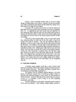
Fig 5.3
Prediction
of
contact
force
variation with time with helical gear.
Prediction
of
Dynamic
Effects
69
-130
-150
ex
c
"5,
-170
10
time
in
milliseconds
20
Fig 5.4
Prediction
of
variation

of
pinion displacement with time.
The
total mesh
force
ff
is
generated
in
line
33 and is
stored
for
plotting
and to be
used
to
calculate accelerations
in
lines
37 to 40.
Accelerations
and
velocities
are
multiplied
by the
time increment
and are
added

to
existing values
to
give
the new
velocities
and
displacements
for the
next
step
of
time.
Results
from the
program
are
shown
in
Fig.
5.3 for the
contact
force
variation
with time.
The
corresponding pinion vibration
is
shown
in

Fig. 5.4.
These
are for an
extreme
case
where
the
gears
are
lightly loaded
(3
kN
at 800 Hz
tooth
frequency) and are
coming well
out of
contact. Once
the
pinion
vibration
is
known, multiplying
by the
pinion support
stiffness
gives
the
pinion
bearing

vibrating forces.
Mean
values
are not
important
as it is
only
the
variation that gives
vibration
and
involute
gears
can
tolerate considerable lateral deflections
though
they
are
highly sensitive
to
misalignments.
An
extra loop
can be put
around
the
program
to
vary
the

tooth
meshing
frequency and
extract
the
vibration
or
peak impact
force
for
each
frequency.
Since initial conditions produce transients,
it is
necessary
to
ignore
the first few
milliseconds
of
response
before
extracting
maxima.
Figs.
5.5
and 5.6
show
the
results

of
such
a
program with
the
typical sudden jumps
70
Chapter
5
in
amplitude when bounce (loss
of
contact) starts
to
occur.
The
mean contact
force
is 3 kN.
With
the
program
as
written there
are a
large number
of
points
to be
computed

when
the frequency is low so it
would
be
preferable
to
start
the
frequency
further
up the
range
if
higher computation speed
is
required.
The
modified program (for
a fixed
mean contact load
of 3 kN) and
provision
for
plotting peak forces
and
pinion support
force
vibrating
amplitude
is:

%
Program
to
estimate dynamic forces under
loss
of
contact AUTO
%
clear;
%
Enter known constants Damping must
not be
excessive
sp =
2e7;
sw
=
6e7;
mp
=
30;
mw
= 70; %
linear
stiffri
and
masses
Kpr=4e6;Kwr=
1.5e7;Iprr
= 20;

Iwrr=90;
% ang
eff.
stiffh
and
masses
bp
=
Ie3;
bw
=
2e3 ; qpr
=1.5e2
;
qwr
=
3e3 ; %
eff. damping
coeffts.
tr=3000;
% fixed
tooth load
for
ddd =
1:40;
%
start
of frequency
loop
freq

=
50 * ddd ;
kk
=
round(20000/freq);
%
steps
for 1
tooth mesh
timint
=
5e-5
; %
time
for
single step 1/20000
sec
predefl
= tr *
(1
/Kpr
+
1
/sp
+1
/sw
+
1
/Kwr);
%

elastic
defi.of
shafts
% and
torsions under steady torque referred
to
contact,
then zero
of
%
input torsion
is
predefl
from
zero force position (ignores contact
defl)
yp=-tr/sp;yw=-tr/sw;rthw=-tr/Kwr;rthp=-yp-yw-rthw;
% set
initial
values
vp
=
0 ;
vw
=
0 ;
revp
= 0 ;
revw
=

0 ; %
velocities
at
mesh
facew=0.
105;bpitch=0.0177;
%
specify tooth geometry
6mm mod
++++
misalig=40e-6;bprlf=25e-6;
%
relief
at 0.5
base pitch
from
pitch point
strelief
=
0.2;
%
start linear
relief
as fraction of bp from
pitch
pt
slicew=facew/21
;tanbhelx=0.18;tthst
=
1,4e

10
;
%
standard value
relst=strelief*bpitch;tthdamp
=
Ie5;
%
eff.value
at
10000
rad/s
Q
=
14++
ss
=
(1:21
);hor
=
ones(
1,21);
%
21
slices
across
facewidth
x = ss -
11
*hor;

%
dist
from
facewidth centre
in
slices
for
tthno
=
1:20;
%
number
of
complete meshes
for
k =
1
:kk
; %
complete tooth mesh
20000/freq
hops ****
ccp
=
yp
+
yw
+ rthp + rthw ; %
interference
at

pitch
pt in m
ccpv
=
vp + vw +
revp
+
revw
; %
relative velocity between gears
for
contl
=
1:4
; % 4
lines
of
contact possible
$$$$$$$$
yppt(contl,:)=x*slicew*tanbhelx+hor*k*bpitch/kk+hor*(contl-3)*bpitch;
rlief(contl,:)=bprlf*(abs(yppt(contl,:))-relst*hor)/((0.5-strelief)*bpitch);
posrel
=
(rlief(contl,:)>zeros(l,2]));
actrel(contl,:)
=
posrel.*
rlie^contl,:)
; % +ve
relief only

inter^contl,:)
=
ccp*hor
+
misalig*x/21
-
actrel(contl,:);
%
local
int
Prediction
of
Dynamic Effects
71
posint
=
interf(contl,:)>0
; %
check
in
local contact
equivint(contl,:)
=
interf(contl,:).*posint
+
posint*tthdamp*ccpv/tthst;
end
% end
contact line loop
$$$$$$$

ffst = sum
(sum(equivint));
%
force
due to
stiffness
and
damping
ff
=
ffst
*
tthst
*
slicew
; % tot
contact
force
is ff
datp
=k +
(tthno
- 1
)*kk;
ffi(datp) =
ff;
%
logs
force
to file

%
total contact
force
>»»»»»»»»»»»
dynamics
accyp
=
-(ff
+
sp*yp
+
vp*bp)/mp;
%
pinion
ace.
linear
accyw
=
-(ff
+
sw*yw
+
vw*bw)/mw
; %
wheel
ace.
linear
accthp
=-(ff+(rthp-predefl)*Kpr+
revp*qpr)/Iprr

; %
pinion
ang
at
mesh
accthw
=
-(ff
+
rthw*Kwr
+
revw*qwr)/Iwrr;
%
wheel
ang at
mesh
vp
=
vp
+
accyp
*
timint;
vw
=
vw
+
accyw
*
timint;

% new
velocities
yp
= yp + vp *
timint;
yw
=
yw
+ vw *
timint;
% new
displ.
pdispl(datp)
=
yp*
1
e6; % to
check loop
progress
revp
=
revp
+
accthp
*
timint;
revw
=
revw
+

accthw
*
timint;
rthp
=
rthp
+
revp
*
timint;
rthw
=
rthw
+
revw
*
timint;
% ang
displ
end
%
next value
of k New
values
of
displ, angles
etc.*****
end
%
tthno loop

end
xzx(ddd)
= 50 *
ddd;
totno=length(ffi);
stff(ddd)
=
max(ffi(100:totno))/1000;
%
peak
after
settling
for 5
millisec
annal
=
fft(pdispl(100:totno));
fftno
=
length(annal);
brgvb(ddd)
=
20*4*
max(abs(annal(2:fftno)))/fftno;
% p-p
value
clear pdispl
iff
end
%main

frequency
loop
figure;plot(xzx,stff);xlabel(
l
Frequency
of
excitation');
yiabel('Maximum
contact
force
in
kN');title('3000N
mean
load');
figure;plot(xzx,brgvb);xlabel('Frequency
of
excitation');
ylabel('Vibrating
force
through pinion bearing p-p');title('3000N mean
load
1
);
end
5.5
Stability
and
step length
The
requirement

for a
short time interval
in the
computing
arises
from the
necessity
to
calculate
for a
time short enough
so
that
a
large spring
force
or
damping
force
is not
allowed
to
"act"
for so
long that
it
over-corrects
for
a
deflection

or
velocity
and
reverses
the
direction.
In
practice this means
selecting
a
time interval which
is not
greater than one-tenth
of the
periodic
time
of the
highest natural
frequency
encountered
in the
system. This
can be
found
either
from a
linear analysis
or
guessed
from the

tooth
stiffness
and the
effective
masses
of the
gears.
72
Chapter
5
20
10
1000
frequency of
excitation
2000
Fig 5.5
Prediction
of
variation
of
maximum contact
force
with
tooth
frequency.
In
the
example given,
the

highest natural
frequency
(when
in
full
contact)
is of the
order
of
1600Hz
so
with
a
periodic time
of
600us,
a
time
interval
of
50u,s
was
taken.
A
test
run
with half
the
time interval
(25us)

quickly
checks that
the
computation
is
satisfactory since there
is no
significant
change
in the
result.
The
other factor which
can
give instability
in a
calculation
is the use
of
a
damping that
is too
high. Since
we
know that
in a
mechanical system
damping
is
stabilising, there

is a
tendency
to try a
computation with
a
high
level
of
damping
on the
assumption that
the
computation will then
be
stable.
The
opposite applies
because
the
very high damping force acting
for a
finite
time
is
liable
to
reverse
the
velocity giving instability.
It is

easy
to
apply
too
high
a
damping
if the
effect
of the
multiplication
by
o>
is
forgotten.
The
product
of the
damping coefficient
and the
contact natural
frequency
should
be
less than
the
mesh contact
stiffness
initially
by a

factor
of
about
10. As
with high spring stiffnesses, reducing
the
time interval step helps
to
give
stability.
If
problems
are
encountered
the
simplest approach
is to
reduce
damping
and
time interval
and if the
system
is
still
unstable
to
check
the
signs

of all
terms
in the
computation.
Prediction
of
Dynamic Effects
73
400
i-
.S
G.
|
I
200
1000
frequency of
excitation
2000
Fig 5.6
Variation
of
vibrating pinion support
force
with tooth
frequency.
5.6
Accuracy
of
assumptions

Assessment
of the
accuracy
of the
assumptions made involves
the
points
mentioned
in
section
4.6
affecting
the
static
T.E
estimates
as
these
factors
still apply. Uncertainties
on
manufacturing errors
are
small though
alignments
are
difficult
to
control. Tooth
stiffness

varies
but has
little
effect
on
the end
result.
3-dimensional
(axial)
effects
should
be
small
with
low
helix
angles
but
gear
body distortions
and
movements
can
have
major
effects.
The
additional factors involved
in the
dynamics case are:

(i)
Inertias
and
moments
of
inertia. These present
no
problems
and are
usually
determined easily
and
accurately.
(ii)
Support lateral
stiffnesses
and
drive
shaft
torsional stiffnesses. These
are
subject
to a
much
greater degree
of
error
as it is
difficult
to

assess
the
effective
lateral
stiffness
of
very short shafts
and the
bearing
stiffnesses
are
susceptible
to
small changes
in
alignments
and
casing
design.
It is
possible
to
measure
stiffnesses
in
situ
but
bearing lateral
stiffnesses
and

their restraining
stiffness
against misalignment vary with
74
Chapter
5
speed, load,
and frequency for
plain bearings
and
with load
for
rolling
bearings.
We
conventionally make
the
assumption that
the
gearcase
is
rigid
but all too
often
this
is not a
valid assumption. Some gearcases
may
deflect
rather easily, reducing

effective
stiffness
at low
frequency.
When
above
a
natural frequency,
the
gearcase bearing housings
may
respond 180°
out of
phase. This gives motion
of the
housing opposing
the
bearing
and
shaft
deflections
and so
there appears
to be an
increase
in
the
support
stiffness
and

natural frequencies
are
higher than
expected.
(iii)
Gear support damping. Damping produces more uncertainty than
any
other
aspect
of the
problem
as is
true
in
most mechanical vibration
engineering.
It is, in
general,
not
possible
to
predict
it and
even less
possible
to
control
it. We are
dependent
on

experience (and possibly
testing)
to
give
a
rough estimate
of the
damping
we
will
get.
The
actual
mechanism
of
damping
in a
machine
is
obscure since material (steel)
damping
is
very
low
(typically
of the
level that would give resonance
amplifications
greater
than 100),

air
damping
is
negligible
and
rolling
bearings absorb
no
energy. Even plain bearings, though
useful
energy
absorbers
at
once-per-revolution
frequency, are far too
rigid
at
once-per-
tooth
frequencies or
above,
so
they absorb little energy. Bolted
or
shrink
fit
joints
are
good
at

absorbing energy
but
there
are few of
these
in
modern designs.
The
most
effective
dissipation mechanism
is
probably
the
radiation
of
vibration energy into
the
flexible
casing because little
of
the
energy returns
to the
rotors.
A
gearbox
which
is
bolted down

to the
ground
can
dispose
of
much energy into
its
foundations
but it is the
energy transmitted into
the
supports which gives
the
troublesome noise
in
most installations.
We are
left
with
the
curious deduction that
an
apparent improvement
in the
internal dynamics
by
altering support
stiffnesses
may be at the
expense

of
radiating more energy into
the
structure
and so
increasing external noise. Lack
of
knowledge
of
support damping
may not be
important since damping only tends
to
dominate
vibration
response
near resonances. Normally drives
are
kept
away
from
resonant
frequencies. If
resonances
can be
avoided,
the
damping
uncertainties
are

less
important.
(iv)
Tooth impact damping. This
is a
very important factor
in
determining
how
far
apart
the
teeth
may
bounce
and the frequency
range over which
there
will
be
trouble. Typically
we
measure impact energy loss
by
generating
an
impact
and
determining
e, the

coefficient
of
restitution,
by
measuring relative velocities before
and
after
the
impact. Since this
is
not
feasible with
gears,
we use the
alternative approach
of finding the
damping
while
the
gears
are in
contact
from the
resonant damping
factor
for the
very high
frequency
modes which
are

associated
with
Prediction
of
Dynamic Effects
75
contact deflections. Dynamic magnification
(Q)
factors
of the
order
of
10
are
typical
for
mechanical
resonances
in
machinery
and
gearboxes
so
we
can
make
a
good guess
at
damping

by
taking
the
peak damping
force
to be 10% of the
peak
elastic
force
during impact. Dividing
by the
natural
frequency
w
n
of the
contact resonance gives
the
damping
force
coefficient.
There
is
another uncertainty
associated
with damping
as we
tend
to
assume

in any
estimates that damping
is
proportional
to
relative velocity.
The
main
reason
for
this
is
that
all
linear analysis
can
only deal with this
assumption
and
estimates
for
hysteretic
damping
or
more complex models
of
damping
become rather complicated
for
simple analysis, whether

by
matrix
(linear) methods
or by
time marching approaches.
In
reality
the
damping
is
probably most accurately
represented
by a
hysteretic model
but we
avoid
the
problem
to
keep
life
simple.
In
the
program
the
damping
is
added with
a

coefficient
tthdamp
which
is
derived
by
taking
the
standard tooth
stiflhess
coefficient
1.4
*10
10
and
dividing
it by a Q of 14 to
give
10
9
N/m/m.
Then since peak velocity
is
ox
if
peak displacement
is x,
assuming
a
resonant

frequency in
contact
of
1600
Hz or
10,000
rad/s,
we get a
damping coefficient
of
10
9
N/m/m
divided
by
10,000
to
give
10
5
N per
unit velocity
per
unit
facewidth
(N
s/m
2
). This
damping

only exists
if the
teeth
are in
contact
so the
logic matrix
(posint)
which
locates
contact
is
multiplied
by the
relative velocity
at the
pitch point
and the
damping coefficient.
The
resulting force
per
unit length
of
tooth
contact
is
turned into
an
equivalent elastic interference

and
added
to the
main
interference
to
give
the
contact
force
at
each
slice.
From
an
academic
perspective this
can be
criticised because
it can
give slight negative values
of
local
contact force,
but the
effect
is
very small
and the
alternative methods

of
modelling damping give much
greater
problems.
The
main
effect
of
uncertainties
in
damping
is
that they alter
the
dynamic
magnification
at
resonances
or
alter
the
possible height
of
bouncing
and
thereby
the
impulsive forces
and
stresses.

However,
the frequency
ranges
in
which trouble occurs
will
be
little
affected
and it is
usually where trouble
happens that
is of
most importance, rather than exactly
how
high
the
stresses
rise.
As far as
estimates
are
concerned,
all
that
can be
done
is to
guess
a

Q
(magnification) factor,
as
suggested above,
on the
basis
of
experience
of
measured values
and
then
use
this value
for the
estimates.
5.7
Sound predictions
The
comments applicable
to
modelling
the
internal dynamics
of a
gearbox apply equally well
to
modelling
the
casing response.

Masses
and
76
Chapter
5
stiffnesses
may be
predicted with reasonable accuracy
but
damping
is a
major
unknown. Unless there have been measurements
on
similar
gearcases
and
installations,
it is
only possible
to
guess
at Q
values.
If
the
casing response
is
modelled
it is

possible, though laborious,
to
estimate
the
total sound power radiated
from the
system
at the
various
frequencies
[1,2].
Then there
are the
complex
effects
of
interference between
the
various sound
sources
to
generate
the
external sound
field.
Uncertainties
of
the
order
of 10 on the

range
of
internal
and
casing damping
factors
mean
that
the
final
result
is
liable
to be
lOdB
incorrect either
way so the
result
may
not be of
much
help
as a 20 dB
range
is
involved.
It is
usually more
economic
to

follow
standard design practice
and
then await practical
tests
on
the
casing.
Predictions
for a
poorly designed casing with large panels
may be
relatively
accurate
but the
better
the
design
of the
casing,
the
more
difficult
it
will
be to
make predictions. Fortunately
the
design rules
for

quiet casings
are
well
known
so it is
straightforward
to
start with
a
good design.
References
1.
Lim,
T.C.,
and
Singh,
R.,
'A
review
of
gear housing dynamics
and
acoustics
literature.'
NASA Contractor Report
185148
Oct
1989.
2.
Fahy, F.J. Sound

and
structural vibration. Academic
Press,
London,
1993.
Measurements
6.1
What
to
measure
As
it is
gearbox noise that
is the
problem,
the
obvious thing
to
measure
is
noise, with
a
microphone placed
in
typical listening positions
around
the
installation. This, however, produces
a
great deal

of
information
which
is
highly
confused.
A
microphone picks
up
combined noise
from all the
panels
of a
gearcase
and the
relatively
low
speed
of
sound
in air
(300
m/s
compared with
5000
m/s in
steel) means that
at a
typical tooth meshing
frequency of 600 Hz

the
wavelength
is 0.5 m. Two
panels vibrating
in
phase 0.25
m
apart
will
produce sound waves exactly
180°
out of
phase.
The
interference between
the
waves will have
a
major
effect
on the
sound
and
small variations
of
position will give
major
changes
in
sound level.

In
addition
if
there
are
other machines
or
walls
near,
then
the
reflections
from
the
surfaces
will
further
confuse
the
measurements.
Fig
6.1
illustrates
the
problem.
The
other
effect
of the
speed

of
sound
is to
delay
the
measurement
and
spread
it in
time.
If, for
example,
the
teeth were bouncing
out of
contact
there would
be a
series
of
impulsive waves reaching
the
gearcase
and
radiating pulses
of
noise.
Path length differences
of the
order

of
only
0.6 m
would
spread
the
"pulses"
over
2
milliseconds.
A
series
of
pulses
at 500 Hz
tooth
frequency
would then appear
at a
microphone
as a
continuous sound,
making
diagnosis more
difficult.
The
interference
and
reflection problems
are

slightly eased
if we use
sound
intensity measurements made very close
to
vibrating panels. Unlike
sound level measurements, sound intensity measures
the
amount
of net
sound
power being transmitted
in a
given direction
and is
unaffected
by
reflections
which
may
greatly increase local sound levels. Conversely, high local power
emissions
may be
subsequently
cancelled
by
another panel acting 180°
out of
phase
(a

dipole
or the
rear
of a
rigid body).
The
disadvantages
lie in the
high
costs
of the
equipment
and the
limitation that
we are
just measuring
the
local
performance
of a
particular resonating panel.
Due to
phasing
effects
high
power radiated
from one
panel could
be
effectively

cancelled
by a
roughly
equal power radiated
at the
same
frequency from a
neighbouring panel
vibrating
180°
out of
phase.
77
78
Chapter
6
gearbox
\
^
'
/ /
7
J
II
\
_^^^B-
I
JftPjffi^Sjffi^^"^"
>
'

)
\
microphone
ESSSSmS^^
wall
Fig 6.1
Sketch
of
setup
indicating
sound reflections
and
multiple paths
to
microphone.
The
further
any
measurement moves away
from the
original source
of
the
vibration, i.e.
the
contact between
the
teeth,
the
greater

the
opportunity
for
there
to be
vibration paths
in
parallel allowing complicated interactions
and
interferences.
If we
want information
as
uncontaminated
as
possible,
it is
desirable
to go
back
as
close
to the
mesh (the original source)
as
possible.
Measuring
on the
rotating
shafts

inside
the
gearbox would give
us
the
clearest
and
most informative measurements
but
since
it is
experimentally
difficult,
this technique
is
only used
for
very special
cases.
Normally
the first
point
at
which
we can get to the
vibration
is at the
bearings
where
we

would
like
to
measure
the
forces coming through
the
bearings,
but can
more easily
measure
the
housing vibration.
Housing vibration
is a
very simple, robust measurement using
standard
cheap accelerometers
and it
gives
a
good idea
of the
levels
at the
interface
between
the
gearbox internals
and the

gearcase.
It is
then easy
to
use a
moving coil vibrator
to find the
local impedances
at the
bearing
housings
so we can
work backwards
from the
observed vibrations
to
determine
the
forces coming through
the
bearings.
In
nearly
all
this work
the
casing system
is
effectively
linear

so we can use
superposition
to
deduce
the
effective
exciting force
at the
bearing.
An
observed
vibration
of
amplitude
b
Measurements
79
with
a
measured combined local
stiffiiess
k
infers
an
equivalent exciting
force
of kb.
Some adjustments must
be
made

for the
vibration
at one
bearing
housing
due to the
excitation
forces
at the
other (three) bearings (see section
16.4).
The
simplicity
of
measurement
and the
fact
that
the
bearing housing
is
usually
the
nearest
we can get to the
trouble source, combine
to
make
the
use of

accelerometers
on the
bearing housing
the
predominant method
of
measurement
for
investigating noise source problems. Using accelerometers
to
roam around
the
casing
or
installation allows
us to
deduce where
the
large
noise-producing vibrations
are
occurring. Measurement
of
transmission error
at
the
gear mesh,
discussed
in
Chapter

7, is
essential
and is
powerful
and
informative,
but
more
difficult
and
requires more expensive equipment.
It
gives
us the
information
about
the
excitation
from the
gears
but not the
information
about
the
dynamic
responses
of the
whole system. Both batches
of
information

are
needed
to do a
thorough investigation
as the
T.E. gives
us
the
original vibration generation
information
and the
accelerometers give
the
casing
and
system
response
information.
6.2
Practical measurements
As
far as
noise measurements
and
deductions
are
concerned there
are few
restrictions
on

measurements. Measurement
of
sound pressure levels
is
easy
since
a
basic (digital) noise meter with analog output jack
[1]
can
cost
less
than £100 ($150)
and the
output
signal,
directly proportional
to
sound
pressure level,
can go
straight into
an
oscilloscope,
a
recorder
or
wave
analyser. Direct viewing
of the

signal
on an
oscilloscope should always
be
used
as it is
very
useful
to get an
idea
of the
character
of a
sound
and
whether
there
is a
simple repetitive pattern. Synchronising
the
oscilloscope
to
once
per rev of
each
shaft
in
turn gives
a
clear idea

of
whether
or not
there
is a
pattern.
The
alternative
of
using
waterfall
plots
is
sometimes less
helpful
especially
if
there
is
regular torque reversal
during
each
rev as
with
a
reciprocating engine.
At
500 Hz, a
typical tooth meshing
frequency,

lum
corresponds
to
Ig
acceleration
so,
since
we can
measure down
to
0.001
g
with
a
standard
piezo-electric
accelerometer
easily, there
are no
sensitivity limitations
at
this
sort
of frequency. A
typical simple circuit
for a
charge
amplifier
(Fig. 6.2)
gives

a
sensitivity
of 22
mV/pC
from 3 Hz to frequencies
above
100
kHz.
A
simple
fixed
gain circuit works well, provided
it is
shielded
from
external
electrical
noise,
and is
extremely reliable
since
there
are no
switches
or
internal
connections
to
give trouble. These advantages more than compensate
for

the
lack
of
adjustment
on
sensitivity.