Gear Noise and Vibration Episode 2 Part 1 ppsx

140
Chapter
9
and
pinion. Frequency analysis
is of
little help since
all frequencies (or
all
multiples
of a
couple
of
very
low frequencies) are
present.
Which
of
these types
of
noise causes
the
irritation depends,
to a
large
extent,
on
what
the
listener
is

expecting.
One
engineer
will
often
expect (a),
(b),
and (d) and
ignore them
but
will
be
highly irritated
by
(c), whereas
another might reject
due to
(b).
One car
driver might
be
irritated
by (a) and
ignore (d), while another would react
the
opposite way. Occasionally,
as
with
a
car,

it is not the
noise itself which irritates
but the
fact
that
the
noise
has
changed
from a
familiar,
accepted
"normal"
noise.
There
is
interaction
in
human
response
between
the
various sounds
and
sometimes
it is
possible
to use the
deliberate addition
of

pitch
errors
in a
drive
to
break
up the
sound pattern. This technique
is
sometimes used
in
chain
drives
if the
customer
is
irritated
by a
steady whine.
9.2
Problem identification
From
what
has
been said
in
section
9.1
the
accurate specification

of
the
problem
is not
always easy. Occasionally
it is a
simple pure tone that
is
heard and,
if a
quick check with
a
sound meter straight into
a frequency
analyser
or
oscilloscope (see section 6.2) confirms that
the frequency is
once-
per-tooth,
diagnosis
is
easy.
Checking
the
character
of the
sound
is a
great help

and if the
sound
is
complex, some
form
of
artificially
generated range
of
sounds
can
help
identify
the
type
of
noise. This
can be
done using predominantly analog
equipment
but it
needs
quite
a
complicated setup
so is
more cheaply tackled
by
generating
a

series
of
repetitive time sequences with
and
without
the
various
errors
in a
standard
PC. The
resulting time series
for
each revolution
is
then
fed via an
output card into
an
audio amplifier
and
loud
speaker
or can
be
played
out on a
sound
card.
The

problem with standard soundcards
is
that
varying
the frequency is not
easy. Reasonable resolution
is
obtained
if
each
tooth interval
is,
say,
30
samples long
and 25
teeth need
750
sample points
per
revolution.
The
various types
of
error
can be
generated
as
(Fig.
9.1):

(a)
1/tooth
errors,
amplitude times
mod
(sin
7tx/30)
gives
the
typical half
sine
wave
of
1/tooth
(for
x
=
1:750
as the
position round
the
revolution).
(b)
Pitch
errors.
These
can be put in as
positive
and
negative

at
arbitrary
positions
of x. The
classic dropped tooth
can be
modelled
as
h
x/750
where
h is the
drop size.
It is
helpful
to be
able
to
either
add or
subtract
a
given pitch error
because
the
audible
effects
are not
necessarily
the

same.
Analysis Techniques
141
T.E
(a)
(b)
T.E
regular
once
per
tooth
^YYYYYYYYYYYYYYYYYYYYYYYYYYYY\
dropped tooth errors
random
pitch errors
one
revolution
Fig 9.1
Models
of
various types
of
noise generated
by
gear drives.
(c)
Modulation. Multiplying
the
sequence
of

1/tooth
errors
by (1+ sin
(27tx/N))
allows modulation
at
I/rev
(N =
750)
or
wheel
frequency (N
=
1300)
or
2/rev
(N =
375)
for a
diesel
or at any
other possible torque
variation
frequency.
(d)
Eccentricity. This
can be
modelled
as e sin
(Ttx/375)

and
added
in but
will
not
alter
the
sound.
It is,
however,
useful
for
demonstrating that
142
Chapter
9
eccentricity
is not
audible unless
it
modulates
the
higher
frequencies
present.
(e)
Random
"white
noise"
can be

added
for
comparison purposes. Again
the
terminology
is
muddling
because
we add
electrical white noise
to
the
input signal
and the
loudspeaker then gives audible noise which
has in it a
random content (noise) which
has
equal amplitudes
at all
audible
frequencies so it is
"white."
Alternatively "pink" noise
with
roughly
equal power
in
each octave
can be

used.
Generally
a
single revolution sequence
in a
program
is
straightforward
in a
language such
as
Matlab. Perhaps
60
revolutions
can be
sequenced
together
to
give runs
of the
order
of
seconds, then
the
sequence
can
be
repeated
to
give

of the
order
of 10
seconds running time. Varying
the
frequency
of
the
sample rate
of the
analog output channel
on the
computer
then
gives
the
effect
of
varying gearbox speed
as
when running
a
gearbox
up
to
speed.
Using
the
original typical T.E.
as the

input
for the
noise does
not
take into account
the
dynamic responses
of the
gearbox
and its
installation.
In
practice, this does
not
seem
to
matter since
it is the
character
of the
sound
that
is
important
and the
customer
will
usually readily
identify
the

"same
sort"
of
sound.
It
is
important
to
identify
the
type
of
problem
because
the
techniques
to be
used
for
analysis depend
on the
type
of
error.
Equally
helpful,
as
previously mentioned (section 6.2),
is the use of a
simple basic noise meter (about

£1007$
150) with
an
analog output
which
can
be fed
directly into
an
oscilloscope synchronised
to
I/rev.
This immediately
gives
a
great deal
of
information about
the
regularity
of the
sound
and
whether
it is
occurring
at
particular points
in the
revolution

or is a
steady
sound.
If
the
microphone information
is
confusing, going
to an
accelerometer
and
checking bearing housing vibration
is the
next move
but
care must
be
taken that
the
main trouble
frequencies
investigated
at the
bearing
are the
same
as
those
being
heard

(and
irritating
the
customer).
9.3
Frequency analysis techniques
Fourier ideas
start
with
the
observation that
any
regular waveform
can
be
built
up
with selected harmonics
with
correct phasing. Fig.
9.2
shows
how
the
first
four
harmonics (all sine waves) added start
to
approximate
to a

saw
tooth wave.
It is
important
to get the
correct
phasing
of the
harmonics
relative
to the
fundamental
or you get a
completely
different
character
of
waveform.
Analysis Techniques
143
1.5
1
0.5
-0.5
-1
-1.5
0.5
1.5
2.5
3.5

time
Fig 9.2
Build
up of
saw-tooth
waveform
with
first
four
harmonics.
The
technique which dominates most (digital) analysis currently
is
Fourier
analysis, usually called
fast
Fourier transform (FFT)
[1]
because
it is
technically
a
computationally more
efficient
number crunching process than
the
classical multiplication technique.
The
details
of the

algorithm
are
irrelevant
but it is
worth noting that routines
prefer
to
have
an
exact binary
series number
of
data points; 1024
was
popular
but
8192
is now
often
used
for
irregular
or
non-repeating vibration.
However,
if a
signal
has
been averaged
to

once
per
revolution then
it
is the
number
of
data points
per
revolution that must
be
used
to get a
correct
answer
and the
sequence should
not be
"padded"
with extra
zeros.
This basic idea
can be
extended
to a
single occurrence such
as a
pulse.
A
pulse

can be
considered
as one of a
repetitive string with
a
very long
wavelength
so
that
the
fundamental
frequency
approaches zero
and
"harmonics"
then occur
at all finite frequencies.
Alternatively,
a
pulse occurs
if
a
large number
of
waves
of
equal,
but
very small, amplitude happen
to all

have zero
phase
at a
single point.
At
that point they will reinforce, giving
a
pulse,
but at all
other places
will
randomly
add to
(nearly) cancel
out to
zero.
Fig.
9.3
indicates
how the
components build
up.
If,
however,
the
components
do not all
have zero phase
at a
single

point
in
time
the end
result
is a
small amplitude random
"white
noise"
vibration.
144
Chapter
9
-2
-0.02
-0.015
-0.01
-0.005
0
time
0.005
0.01 0.015 0.02
Fig 9.3
Seven components coinciding
to
give
a
pulse.
The
reverse process involves using

a
sine wave
as a
detector
by
multiplying
the
signal under
test
by a
sine wave
of frequency
co
(and unit
amplitude)
and
averaging
(or
smoothing)
the
resulting signal.
Any
component
not at co
will
average
to
zero
over
a

long period
since
the
product
is
negative
as
much
as it is
positive (Fig. 9.4),
but if
there
is
a
component
A
sincot
hidden
in the
signal, then
the
output
is A sin
cot,
which
averages
to a
value
A/2.
Initially

the two
signals
in
Fig.
9.4
were
in
phase
so
they gave
a
positive product,
but
then they became
out of
phase
and
gave
a
negative with cancellation over
a
long period.
Testing
at all frequencies and
with both
sin and
cosine detects
all
possible
components.

This
classical
approach
involved
testing
over
a
longish
time
scale
(with
limits
of
integration
-
oo
to +
QO)
and
returned
an
amplitude
of a
particular harmonic.
Current digital techniques work
to a
finite time scale
(or to be
precise,
a finite

number
of
samples)
so
they give
a
slightly
different
form
of
result.
A finite
number
of
points
(formerly
1024) leads
to the
calculation
of
the
total energy
within
a
narrow
frequency
band whose width
is
determined
by

the
number
of
sample points
or the
time scale
of the
test.
As
with
all
frequency
analysis,
in
theory
at
least,
the
longer
we sit and
test,
the
more
accurate
the
result
and the
narrower
the
measurement band possible. This

is
because
the
longer time scale allows
the
signals
to
change phase
if
they
are
not
exactly
the
same
frequency.
Analysis
Techniques
145
Fig 9.4
Result
of
multiplying
two
slightly
different
frequencies.
power
effective
bandwidth

power distribution
at all frequencies
frequency
Fig 9.5
Frequency analysis with
finite
bandwidth.
146
Chapter
9
ampl
background
noise
lines
frequency
Fig 9.6
Type
of
line spectrum obtained with rotating machinery.
The
idea that
we are
inevitably measuring power
in a
narrow band
rather than
a
finite
amplitude
of a

component leads
to the
mental picture
in
Fig. 9.5. Here
we
have many components
at a
range
of frequencies and the
effect
of the
analysis techniques
is to
model
an
almost perfect narrow band
pass
filter
which
lets through only those components
within
the
band
and we
can
then measure
the
resulting power.
The

resulting output
from the
analysis
is in the form of
power
in
each
frequency
band
and
this
is
converted
to
power
per
unit bandwidth called
power spectra] density (PSD), originally
in the
effective
units
of
(bits
2
/sample
interval)
but
usually
converted
to

volts
2
/Hz
or
reduced
to
volts/^Hz.
This
form
of
presentation works well
for
random phenomena
and for
most natural
processes
such
as
wave motion
at sea
where
all frequencies
exist.
Halve
the
bandwidth
(by
altering
the frequency
scale)

and we
detect half
the
power
so the
power
spectral
density (PSD)
remains
the
same.
Unfortunately,
for
rotating machinery
and
gears
in
particular
we find
that there
are a
limited number
of frequencies
present. These
are
exact
multiples
of the
once-per-revolution
frequencies of the

system and,
in
general,
no
other
frequencies
exist apart
from
some minor background noise
and
some
very small components associated with
the
meshing cycle
frequency.
This
type
of
spectrum
is
usually called
a
line spectrum,
as
opposed
to a
continuous
spectrum,
and the
"power"

in
each
line
is
concentrated into
an
extremely
narrow
frequency
band (Fig. 9.6).
A
line
will
be at 29
times
per
revolution
and at
29.1/rev
there
is
technically
no
power though there
will
generally
be
power
at 28 and
30/rev

due to
modulation
of the
29/rev
at
once-per-rev.
For
Analysis
Techniques
147
this type
of
spectrum
if we
halve
the
bandwidth
the
PSD.
will
double since
all
the
power resides
in an
extremely narrow line, well within
the
width
of a
normal

band.
Some
commercial equipment expects
the
user
to be
measuring line
amplitudes
(in
volts)
but
most equipment expects
to be
measuring PSD.
(in
volts
2
/Hz).
Unfortunately,
it is
customary with both
to
give amplitudes
in dB
so it is
important
to
check whether
a
reading

is 25 dB
down
on 1 V
(line)
or
on
1
volts
2
/Hz
(continuous).
If, as
usual, handbooks
are
uninformative,
then
altering
the
timescale
with
a
single
frequency
input
from an
oscillator will
give
a
quick check
on

which type
of
readout
is
being given.
It
sometimes
happens that those manufacturing
and
selling
the
equipment
are not
aware
of
the
difference
between
the two
types
of
spectrum.
Conversion between
the two
types
of
readout
is not
difficult.
Take

a
readout
of-20
dB on
Ivolts
2
/Hz
with
a
total bandwidth
of
10,000
Hz and 400
lines
in the
spectrum. Each
"line"
is 25 Hz
wide
and the
power
is
0.01
V
2
/Hz
so the
total power
in
that spectrum band

is
0.25
V
2
,
which
corresponds
to a
line amplitude
of 0.5 V. In
contrast,
if the
reading
was -20 dB on
amplitude
the
voltage would
be
0.1
V and the PSD
would
be
0.01
V
2
/25
Hz,
i.e., 0.0004
V
2

/Hz
or
0.02
VA/Hz,
which
is -34 dB. The
only time
the two
readings
would
agree would
be if the
bandwidth were
1 Hz. In
practice
the
units
may
be
given
in g
acceleration,
mm/s
velocity
or urn
displacement instead
of
volts
but the
conversion principle

is the
same.
Previous analog equipment
for frequency
analysis worked
on the
completely
different
principle
of
having
a
variable
frequency
tuned resonant
filter
which scanned slowly
up
through
the
range. This method
is
slow,
expensive
and not
very discriminating
and
requires long vibration traces
for
analysis.

It
also
has the
disadvantage that tuned
filter
circuits
do not
respond
rapidly
to
changes
in
vibration level. There
is a
digital convolution
equivalent which
can be
used
as a
band pass
filter
(when modulation patterns
are
of
interest)
to
extract
a
neighbouring group
of frequencies, as

occasionally
happens with epicyclic gears,
but it is
rare
for
this
to be
required.
When
a frequency
analysis
is
carried
out on a
vibration
or
T.E.
the
band width
of the
resulting display
is
controlled
by the
testing
time. Testing
for
1 sec
would give
a

bandwidth
of 1 Hz for the
output graph whereas
a
test
for
0.1
sec
gives
10 Hz
bandwidth. This bandwidth
may be
unfortunate
if it is
too fine so
that there
are
several lines associated with
a
particular
frequency
such
as
1/tooth.
The
answer
may be
correct
but it
makes comparisons

between
different
gears
difficult
or may
give deceptive answers
if the
tooth
frequency
of
interest happens
to lie on the
borderline between
two
bands
as
half
the
power will appear
in
each band.
148
Chapter
9
One
possibility
is to
reduce
the
test time since halving

the
length
of
record
will
double
the
band
width
but
this
may
mean that
the
test
is for too
short
a
time
to
give
an
average value over
a
whole revolution
or
longer.
A
preferable alternative
is to

carry
out the frequency
analysis with
the
original (long) record then take
the
resulting Fourier analysis
and add
bands
in
groups.
If the
original record
was for 10 s the
bandwith would
be
0.1
Hz and
adding
10
bands would widen
the
bandwidth
to 1 Hz. The
addition
is an
addition
of
power
in the

bands
so the
modulus
of the
result
in a
given band must
be
squared,
the
band powers
added,
then
the
root taken
of
the
sums. This
is
simply
achieved
in
Matlab
by a
short subroutine such
as
rrf=4*(fft(RSTl))/chpts;
%
original record
RST1

p-p
values
trrf
=
abs(rrf(2:1001));
%
knocks
out DC and
gives modulus
pow
=
trrf.*trrf;
%
squares each line
firth =
sum(reshape(pow,10,100));
%
adds
10
lines
to
give
1 Hz
band
sqfr
=
sqrt(frth);
%
gives
p-p

values
for
10
lines
9.4
Window effects
and
bandwidth
One
side
effect
of
finite
length digital records being used with
frequency
analysis
is
that
the
sudden changes
at the
ends cause trouble.
In
Fig. 9.7, with
a finite
window length
L, frequency
analysis
of
curve

A
will
give
an
exact twice
per L
sine component
and no
others,
and
curve
B
will
give
an
exact twice
per L
cosine component
and no
others.
Curve
C
gives trouble
because
the
actual
frequency,
1.2
times
per L

cannot
exist
in the
mathematics, which
can
only
generate integer multiples
of
frequency
1/L.
The
result
of a frequency
analysis
on
this wave
is
that
the
answer contains D.C.
and
components
of all
possible
harmonics
of
1/L.
The
result obtained
is

exactly
the
same
as
that obtained
by
analysing
the
repetitive
signal shown
in
Fig. 9.8.
To
overcome this problem
in the
general
case
of an
arbitrary length
record taken
at
random
from a
vibration
trace,
it is
necessary
to
multiply
the

original vibration wave amplitudes
by a
"window"
which gives
a
gradual
run
in
and run out at the
ends (Fig. 9.9).
This eliminates
the
sudden changes
at the
ends
and
greatly reduces
most
of the
spurious harmonics generated
as a
consequence. There
are
various window
shapes
used,
with
the
Hanning
window being

the
most
common.
The
various standard windows
and
their characteristics
are
described
by
Randall
[2].
The
side
effect
of
using
a
window
is
that
the
effective
length
of the
sample
is
rather
shorter
than

the
total length
so the
total
power
within
the
window
is
reduced
and
correction
is
made
for
this
within
the
standard programs.
Analysis
Techniques
149
1
0.8
0.6
0.4
0.2
0
-0.2
-0.4

-0.6
-0.8
-1
6 8
window
length
L
10
12
Fig 9.7
Finite length records showing
end
effects.
f
0.5
-0.5
-1
10 20
time
30
Fig 9.8
Equivalent continuous record
for
short sample.
150
Chapter
9
original
signal
window

shape
signal
finally
analysed
Fig
9.9
Application
of
^window"
to
remove sudden transients
at
ends.
When
finding
transfer
functions,
the
same window
is
used
for
both
signals
so the
ratio
is
unaffected.
If
no

window
is
used
we
refer
to a
"rectangular"
window
so the
test
data
is not
changed
at the
ends. This
is
legitimate (and desirable) either
when:
(a) The
signal
is a
transient which starts
and
finishes
at
zero
(as
when
impulse testing
a

structure)
or
(b)
The
signal contains only exact harmonics
and so
each harmonic
component
starts
and
stops
at the
same height with
the
same slope
and
the
repeated signal (Fig.
9.10)
would
be
smooth
and
continuous.
Analysis
Techniques
151
vibr
revolution
Fig

9.10
A
signal that
is
correctly repetitive.
This second condition applies when
the
signal corresponds
to an
exact revolution
of a
shaft
and has
been obtained
by
time-averaging (without
jitter
or
smearing problems).
OdB
o
Q.
CO
0>
changeover
frequency
I
lower
band
upper

band
frequency
Fig
9.11 Problem
of
spectrum line
at
borderline between
two
filter
bands.
152
Chapter
9
The
other
effect
of
finite
signal length
is the
limited sharpness
of the
bandwidth
cutoff.
Fundamental theory gives
the
practical working rule that
frequency
resolution

on a
record
B
seconds long cannot
be
better than
a
frequency
of
1/B
Hz so a 2
second long record cannot discriminate
to
better
than
0.5 Hz.
Fig.
9.11
indicates (exaggerated)
the
result
of
this
on the
effective
filter
shape
of a
pair
of

neighbouring bands
or
lines
in the FFT
spectrum.
If
we
then have
a
line
in the
machinery spectrum
as
shown,
it
will
not
totally
appear
in
either band
but
roughly half
the
power
will
be in
each band, giving
a
slightly deceptive impression

of
amplitude. Changing
the
bandwidths
may
straddle
the
line
and
show
the
full
amplitude,
but it may be
necessary
to
read
the two
powers
and add
them
by
hand. This
may
produce complications
if
there
are
other significant vibrations
at

neighbouring frequencies.
Another
technique sometimes mentioned
is
correlation
(or
whitewashing)
which consists
of
multiplying
a
signal amplitude
at
each point
by
a
signal
at a
(variable) time
T
later
and
summing
the
result which
is
then
plotted against
\.
This technique

is
cumbersome
but
determines whether
there
is
something
"interesting"
happening with
a
delay time
T. In the
case
of
any
rotating machinery
we
already know that
"interesting"
things happen
1
rev
later
so
this technique
is of
little help
and
instead
we use

time averaging,
which
is
much more economical
of
computing
effort
and
more powerful
as
well
as
being faster.
9.5
Time
averaging
and
jitter
Time averaging
was
mentioned
in
chapter
8 as a
method
of
compressing
the
amount
of

information
that
was
stored
but has a
much wider
range
of
uses.
In
a
gearing context
the
great
use of
time averaging
is to
eliminate
or
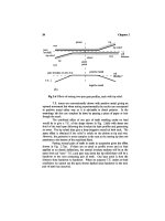
reduce unwanted vibrations. Taking
the
case
of an
in-line
gearbox, sketched
in
Fig.
9.12,
we
have three

shaft
speeds,
input
A,
layshaft
B and
output
shaft
C. If we
suspect
a
dropped-tooth
pitch error problem
on the
output
shaft
C
and
have
an
accurate
I/rev
marker
on
shaft
C we can
time-average
the
T.E.
or

vibration
at the
repetition frequency
of
shaft
C. At
each revolution
of
shaft
C we
read
the
noise, T.E.
or
vibration level
at
perhaps
500
points taken
consistently round
the
revolution.
A
revolution
is
comprised
of 500
data
"buckets"
and on

each
rev the
reading
is
added
to the sum of
previous
readings
in
that
"bucket"
(i.e.,
at
that position round
the
rev).
If we
take
the
sum
of 256
revolutions
and
divide
the
resulting totals
by
256,
our
scale factor

is
unaltered
and we
have obtained
an
average vibration.
Analysis Techniques
153
input
A
I
B
output
layshaft
Fig
9.12 Sketch
of
in-line gear drive with three
shafts.
All
vibration related
to the
output
shaft,
such
as an
output gear pitch
error,
will
repeat

in
exactly
the
same place round
the
revolution
so it
will
remain
unaltered
in
size.
All
other non-synchronous, intermittent, random,
or
irregular vibration will behave like random vibration
and
average
to
zero.
Even
powerful
vibration such
as
engine inertia
and firing
effects
from a
4-cylinder
engine

will
be
non-synchronous
for the
ouput
shaft
(though
synchronous
for the
input
shaft)
and
will
be
spread
out
round
the
revolution
leaving mainly those vibrations associated with
the
output gear (and prop
shaft
and
hypoid
pinion
if fitted).
A
very
narrow

firing pulse consistently
at one
point
on the
input
shaft
will appear
at
each tooth interval
on the
averaged
layshaft
trace reduced
in
amplitude
by a
factor
equal
to the
number
of
teeth
on the
layshaft.
Fig.
9.13
shows
the
effects
of a

consistent narrow
firing
pulse
of
height
H if it is
on
the
"averaged"
input
shaft
and if it is on a
neighbouring
shaft,
in
this case,
the
layshaft.
Additional
to the
benefit
of
extracting
the
information associated
with
a
particular
shaft
rotation, averaging increases

the
accuracy
of the
readings
and
improves
the
resolution.
If
the
original
full
scale
(10
volts)
is
represented
by 12
bits, then,
after
averaging,
the
total
can in
theory
be up to
12
bits
x 256
which

is 20
bits size
so
after
averaging
we can
have
a 20 bit
range. This seems
to be
impossible since,
if
full
scale
is 10
volts then
originally
1 bit is 2.4 mV, and it
does
not
seem possible
to
achieve
a
resolution better than 0.01
mV.
In
practice this
can and
does happen

although
only
if
there
is
extra random vibration present.
For
some accurate
measurements
a
"dither"
vibration
[3] is
deliberately added
to
increase
accuracy
of the
averaged signal
and to
give resolution
to the
equivalent
of
better than
1 bit on the
original measurement.
In
the
case

of a
gearbox
we
have plenty
of
extra non-synchronised vibration around
so we do not
have
to
bother adding
in the
dither.
154
Chapter
9
Due
to the
averaging
process
the final
averaged result
is
much more
accurate than
the
original
"noisy"
measurements
and
frequency analysis

is
correspondingly
more accurate
and
reliable.
An
averaged signal, exactly
synchronised
to
I/rev,
will
finish
at
exactly
the
same position
as it
started
and
can be
analysed
by
FFT
using
a
"rectangular"
window
and
hence using
all the

information
fully.
The one
revolution
of
averaged information
is
equivalent
to an
infinite
number
of
repetitions
of
that revolution.
The
question arises
as to how
many revolutions
is
necessary
or
desirable
to
average
to get a
"good"
result.
As
usual,

the
answer depends
on
the
"noise"
around, both
in
level
and
character.
ampl
response
after
averaging
is
the
same
as the
original
pulse
H
one
revolution
of
input
shaft
time
ampl
response
after

averaging
at
input
frequency
height
H/N
one
revolution
of
layshaft
time
Fig
9.13
Effects
of
averaging
at
once-per-rev
of
input
shaft
and of
layshaft.
Analysis Techniques
155
Whether
audible, mechanical
or
electrical, random noise which
is

comparable
in
size
to the
signal
of
interest
is
likely
to be
reduced
to
negligible
importance (1%)
if we
average
128
cycles.
If,
however,
the
noise
is 20 dB
greater than
the
signal
we may
have
to go to
1024 averages

but
this,
fortunately,
is
rare.
When
the
"noise"
is due to
pitch errors
on a
mating
gear,
then
the
requirement
is
slightly
different.
By
definition,
the sum of all
adjacent
pitch
errors
on a
gear must
be
zero since, otherwise,
we do not finish a

revolution
where
we
started.
If,
then,
one
selected
tooth
on a
pinion mates once with
every
single tooth
on a
wheel (with
N
w
teeth) then
the sum of all the
errors
must
be
solely
N
w
times
the
error
on the
pinion tooth, since

all
wheel pitch
errors have added
to
zero.
To get the
best averaging
on the
pinion
it
should
do
an
exact multiple
of
N
w
revs
(i.e.,
an
integral number
of
complete mesh
cycles). (This assumes that,
as
usual, there
is a
hunting tooth.)
So,
with

a
single mesh
of 19
teeth (input)
to 30
teeth (output)
we
need multiples
of 30
revs
of the
input
to
give complete meshing cycles
and 120
revs would give
a
good result
and
reduce random noise
effectively.
This meshing cycle idea
gives
an
excessive requirement
if
there
are two
meshes,
as

happens with
a
layshaft
(B in
Fig.
9.12)
with 19:29
at
input
and
23:31
at
output.
For a
complete
meshing cycle
the
layshaft
would have
to do 19 x 31
revs
and 589
revs would take rather
a
long time
and
require some
300,000
data points.
There

is an
exception
to the
basic idea that time averaging separates
occurrences
on two
meshing
shafts.
Regular
1/tooth
and
harmonics appears
on
both
the
pinion
and
wheel averaged traces since
the
steady component
of
1/tooth
averages
up
consistently.
In
both averaged traces
the
regular
1/tooth

and
harmonics components associated with both
shafts
will appear together
with
any
irregular tooth components
due to the
particular
shaft.
Time
averaging appears
to be, and is, a
very
powerful
and
useful
tool
for
rotating machinery,
and for
gear drives
in
particular,
but as
with
all
techniques there
are
liable

to be
problems
or
difficulties.
The
major
problem
is
associated with
"jitter"
or
"smearing"
and is
due
to
variation
in
speed
of
rotation.
The
start
of a
revolution
is
given
by an
accurate
I/rev
pulse

and
with typically
500
data samples
per rev the
starting
position
is
located consistently within 0.2%
of a rev
(0.72°
). If we
have
50
teeth
on the
gear
and are
primarily interested
in
1/tooth
(and harmonics)
noise then
a 1%
variation
in
speed between
one
revolution
and

another would
mean
that
by the end of the
revolution
two
50/rev waves recorded
at the
same
sampling
rate
(in
time) would have moved 180°
in
phase relative
to one
another.
If, at the
start
of the rev
they were adding, they would
be
cancelling
each other
by the end of the
rev.
A 1%
speed change
is
unlikely

to
occur
within
a
revolution
or on
successive
revolutions
but
might occur over
50
revs
156
Chapter
9
which
is the
sort
of
order
of
number
of
revs over which
we
might average
signals.
Fig.
9.14
indicates

the
"smearing"
effect
and
shows
how the
observed averaged amplitude reduces
as the
signals move
out of
phase with
the
speed variation, which
in the
case shown
has
given cancellation with
180°
phase
shift
half
way
round
the
revolution.
The
jitter
effect
causes
trouble

because
we
sample
at a
constant rate
in
time whereas
we
wish
to
sample
at
constant angular positions round
the
revolution.
On a
test
rig
this could
be
achieved
by
fitting
an
additional rotary encoder (with
512
lines)
and
sampling
the

vibration signal when demanded
by the
next encoder line. This technique
is
rather
too
cumbersome
for
general use.
one
revolution
ex
£
slower
revolution
averaged signal
Fig
9.14
Effect
of
speed variation
on
time averaged signal.
Analysis
Techniques
157
An
alternative
to
physically

fitting an
encoder
is to
work back
from
when
the
I/rev
pulses occurred
(in
time)
to
exactly when
the
samples should
have
been taken (assuming constant speed during
the
revolution),
and
then
use
relatively complex interpolation routines
to
estimate what
the
vibration
reading
would have been
if the

sample
had
occurred exactly
at the
"correct"
time. Again this
is
excessively cumbersome
for
normal use.
It is
usually less
effort
(in
total)
to
restrict data logging
to
times when
the
speed remains
reasonably steady over
a few
seconds.
An
interval counter reading
rev
times
from the
I/rev

sensor
and set to
10~
5
seconds
resolution
is
usually
useful.
An
alternative technique
is to
have
two
separate
sensors,
half
a
revolution apart
and
average
on
each separately, using
only
the first
half
of
each
rev and
halving

the
time available
to get out of
phase.
Yet
another, better, approach
is
to
carry
out the
time averaging analysis working backwards
from the
timing
pulses
to
reduce smearing
in the
latter half
of the
rev,
as
well
as
working
forwards
from the
pulses
to
reduce smearing during
the first

half
of
the
rev. This
is
relatively easy
to do in the
analysis routines
and
comparison
of
the
"forward"
and
"backward"
averages gives
a
clear indication
of
whether
there
are
serious jitter problems.
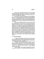
9.6
Average
or
difference
It
is
easy

to get
carried away
by the
power
and
usefulness
of
time
averaging
but
occasionally
it is not the
average that
is
important.
A
classic
case
occurs with internal combustion engines where
we are
less interested
in
the
steady
firing
pulses
from the
(four)
cylinders than
in the

variation
of the
pulses
due to
irregularities
in
carburation
or
turbulence. Correspondingly,
in
gear drives
we may be
interested
in
variations
of
noise pattern
from the
steady
state because human hearing
is
very sensitive
to
small modulations
or
variations
from
regularity.
Irregular variations
in

gear drive noise
or
vibration
can
occur
for
several
reasons.
Intermittent interruptions
in oil
supply
can
have some
effect,
or
alignment variations,
due to the
cage
of a
rolling bearing beginning
to
break
up, can
modulate
the
signal. External variations
due to
variable load
will
influence

noise,
especially
if
teeth
are
allowed
to
come
out of
contact,
or
occasionally dirt
or
debris passing through
the
mesh
will
give transient
vibration.
Hull
twisting
on a
ship
may
distort
the
gear casing
and
alter
alignments

of the
meshes.
For any
problems
of
this type
an
effective
method
is to
compute
the
time
averages
for
both input
and
output
shafts
and
subtract
the
averages
from
the
original
signal
so
that what
is

left
is the
variation
from
average
or
"normal"
signal. Care
is
needed
not to
subtract
the
tooth
frequency
components twice
as
they appear
in
both averages.
The
variation
from
158
Chapter
9
average
can
then give
an

indication
of the
problem
cause,
especially
if
there
is
an
external load
or
speed variation.
9.7
Band
and
line filtering
and
resynthesis
In
many vibration signals there
are
present vibration components,
often
quite large, which
are
irrelevant
to the
investigation.
It is of
little help

to be
told that there
is a
large component
at
21
times
per
revolution
if we
already know that there
are
21
teeth
on the
gear
and
that
the
problem
is not at
tooth
frequency.
Similarly
a
component
at
mains
frequency (or
harmonics)

is
likely
to be
electrical noise
or
drive torque
fluctuations.
It
may be
much
easier
to
analyse
or
assess
the
time signal
if
these
expected components (which
are
legitimately present)
are
removed
from the
signal.
Originally
the
analog methods employed
for

this
involved
either (Fig.
9.15)
(a)
notch
filters
which were
often
for
mains interference,
or
(b)
"band
stop"
filters to cut out a
range
of frequencies,
typically
an
octave.
These helped
but
were
of
limited performance
and
could
not
deal

with
any
subtleties
in the
signals. Digital methods
are
much more
powerful
and
flexible
and now
dominate
the field.
Digital
filters can
give extremely
high performance
high
pass,
low
pass,
band pass
or
band stop performance
to
"clean
up" a
signal
by
removing known, irrelevant components.

response
notch filter
problem
frequency
band
stop
filter
frequency
Fig
9.15 Response
of
analog notch
and
band stop
filters.
Analysis
Techniques
159
They
work
by
convolution, multiplying
the raw
signal
by the filter
impulse
response,
and
involve
a

large number
of
computations,
so it is
difficult
to
achieve high
speeds
at low
cost.
The
alternative, line elimination
and
resynthesis,
is
based
on the
standard
FFT
routines which
are
fast
and
efficient
and can be
easily
programmed
in
Matlab
[4] or a

similar language.
The
vibration trace,
whether
raw
signal
or
rev-averaged signal,
is
analysed using
an FFT
routine
(a
one-line instruction). Then either
(a)
known
lines
which should
be
there
are
removed automatically
or
(b) the frequency
analysis
is
displayed
and the
'legitimate'
lines

to be
eliminated
are
chosen
by the
operator
or
(c) all
lines above
a
certain (absolute) amplitude
are
removed (this
is the
easiest option
to
program
but
involves
an
arbitrary choice
of the
critical
level).
For
each
frequency in a
real signal there
are two
lines

in the FFT
because
frequencies
always appear
as
conjugate complex pairs
in the
analysis.
original
signal
time
difference
signal
Fig
9.16 Subtraction
of
regular signal
from
test signal
to
emphasise changes.