Gear Noise and Vibration Episode 2 Part 5 pps

220
Chapter
13
I
a
roll
tip I
tip
base
pitch
pure
involute
tip
purb
involute
tip
tip
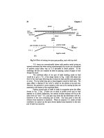
Fig
13.4 Sketch
of T.E
effects
at (a)
correct centre distance
and (b)
extended
centre distance.
Fig.
13.4
shows
diagrammatically
the

difference
between
two
pairs
of
teeth meshing
at
correct
and
extended centres
to
give
the
same changeover
points.
The
test requirement
is
then
to
decide what
increase
in the
centre
distance
will
give crossover points
in
exactly
the

same positions
up the
profiles
of
the
gears
as
when handing over contact under loaded conditions.
The
requirement
is to find the
exact positions
up the
profiles,
not
along
the
roll pressure line, where handover occurs
for the
original contact
geometry
and
match these
to the
handover points
at
extended centres. This
is
an
iterative calculation

and it is
simplest
to use a
computer routine
to
assist
the
process.
%
program
for finding
centre distance change
for
contact ratio
2
%
gears
for TE for
changeover. Work
in
terms
of
nominal module
1
phio
=
18*2*pi/360
; %
design pressure angle
18

at
contact ratio
2
nl
=
32 ; %
number
of
pinion teeth
n2
=
131
; %
number
of
wheel teeth
brl
=
nl*0.5*cos(phio);
br2 =
n2*0.5*cos(phio);
%
base
radii
psil
=
(tan(phio)
+
2*pi/nl)
;

psi2
=
(tan(phio)
+
2*pi/n2);
%
determine unwrap angles
psi at
changeover points assuming both
% are 1
base pitch away
from
pitch point
%
these
unwrap angles must
be the
same
for
extended test
to be
% the
same points
on the
flanks
but
will
occur
at
roughly

% 0.5
base pitches away
from the
pitch point
High Contact Ratio Gears
221
%
take
first
approximation
to new
pressure angle
phil
as due to
%
centres moving
1
module apart
so
phil
=
acos(cos(phio)*(brl+br2)/(brl+br2+cos(phio)));%
new
angle
%
then calculate distances
from
pitch point
to
changeover points

%
divided
by
original base pitch
rl
=
(brl*psil
-
brl*tan(phil))/(pi*cos(phio));
% new
pressure angle only original base radius real
r2
=
(br2*psi2
-
br2*tan(phil))/(pi*cos(phio));
conratio
=
rl + r2;
disp('angle
rl r2
contact
ratio')
disp([phil
rl r2
conratio])
%
line
18
phi2

=
input('enter
new
pressure angle
');
%
****
rl
=
(brl*psil
-
brl*tan(phi2))/(pi*cos(phio));
r2
=
(br2*psi2
-
br2*tan(phi2))/(pi*cos(phio));
conratio
= rl + r2;
disp(
f
angle
rl r2
contact
ratio')
disp([
phi2
rl r2
conratio
])

phi3
=
input('enter
new
pressure angle
')
; %
****
rl =
(brl*psil
-
brl*tan(phi3))/(pi*cos(phio));
r2
=
(br2*psi2
-
br2*tan(phi3))/(pi*cos(phio));
conratio
=
rl + r2;
dispC
angle
rl r2
contact
ratio')
disp([phi3
rl r2
conratio])
%
Iine28

%
calculate increase
in
centre distance
from
original
incr
=
(brl
+br2)*(l/cos(phi3)
-
l/cos(phio));
%
modules
disp('centre
distance increase
modules')
disp(
incr)
The
programme assumes that
the
original crossover points were
placed symmetrically
one
base pitch away
from the
pitch point
and
calculates

the
involute unwrapping angles
to
these
points.
When
the
centre distance
changes
the
only factors that remain
the
same
are the two
base radii
and the
two
unwrap angles
to the
correct crossover points.
The
approach
and
recess
distances
after
the
centre change will normally
not be
equal.

After
the first
guess
at the new
pressure angle only small changes
are
needed
to
adjust
the
angle
(in
radians)
to
give
the
contact ratio exactly
1.
If
the
original design
was not
symmetrical about
the
pitch point
the
original design values
of the
unwrap angles
psil

and
psi2
to the
crossover
points should
be
used.
222
Chapter
13
References
Gregory, R.W., Harris, S.L.
and
Munro, R.G.,
'Dynamic
behaviour
of
spur
gears.'
Proc.
Inst.
Mech. Eng., Vol. 178, 1963-64, Part
I, pp
207-226.
Leming,
J. C.,
'High
contact ratio (2+) spur
gears.'
SAE

Gear
Design,
Warrendale,
1990.
Ch
6.
Yildirim,
N.,
Theoretical
and
experimental research
in
high contact
ratio spur gearing. University
of
Huddersfield,
1994.
Munro, R.G.
and
Yildirim,
N.,
'Some
measurements
of
static
and
dynamic
transmission
errors
of

spur
gears.'
International Gearing
Conf.,
Univ
of
Newcastle upon
Tyne,
September 1994.
14
Low
Contact Ratio Gears
14.1
Advantages
Conventional
industrial gears tend
to use the
standard
20°
pressure
angle
and
standard proportions
and
thus encounter undercutting problems
when
the
number
of
pinion teeth

falls
below about
18.
If
gears
are
highly
stressed they will normally
be
carburised
and the
standard
AGMA2001
or ISO
6336 calculations
will
typically give
a
so-called
"balanced" design
at
about
27
teeth. This means that there
is an
equal likelihood
of
failure
by
flank

pitting
or
by
root cracking.
In
practice
as
root
failure
would
be
disastrous,
it is
normal
to
have
considerably less than
27
pinion teeth
to
make sure that root breakage
is
ruled
out. This leads
to
most standard spur designs having between
18
and 25
pinion
teeth

and
typically having
a
nominal contact ratio about
1.6.
Alternatively
we can
still
get
involute meshing with much lower tooth
numbers
if we are
prepared
to use
non-standard teeth
on the
pinion. Tooth
numbers
of 13 or
11
are
common
on the first
stages
of
small, high reduction
gear boxes
and the low
tooth numbers allow larger reduction ratios.
The

designs
use
increased pressure angles typically
of 25° and are
"corrected"
so
the
pitch circle
is no
longer roughly
55% of the way up the
tooth
but is
only
about
one
third
of the way up the
tooth when meshing
with
a
large wheel.
For
two
equal gears meshing
the
practical
limit
is
about

9
teeth
and
Fig. 14.1 shows
two
such gears
in
mesh.
For
pinion
and
large gear
or the
ultimate
pinion
and
rack meshing
the
practical limit
is
down
to 7
teeth. Again
the
pressure angle
is 25° and the
teeth
are
relatively narrow
at the

tips.
The
theoretical contact ratio
for
these
gears
is
about 1.05
to 1.1 but
this nominal
value
does
not
allow
for the
relatively large contact area. Fig.
14.2
shows
the
geometry
for a
standard design
which
is
used
on oil
jacking rigs where very
large loads must
be
taken

but
pinion diameters must
be
minimised. These
seven tooth
gears
with modules
of the
order
of 100 mm
(0.25
DP) are
used
with
racks either
5" or 7"
facewidth
to
lift
the
high loads
of oil
jacking
platforms
for use in
waters
up to
several hundred
feet
deep.

The
loads
on
each
tooth
are
then
of the
order
of 500
tonnes
and
dozens
of
meshes work
in
parallel.
Fig. 14.3 gives
an
expanded view
of the
contacts near
the
changeover
point
and it can be
seen that there
is
very little overlap when there
are two

pairs
of
teeth
in
contact.
223
224
Chapter
14
Fig
14.1 Shapes
of two
meshing
gears
with nine teeth
and 25°
pressure angle.
As
can be
seen
in
Fig. 14.3 with
the
contact
ratio only slightly
greater
than
1,
contact
is

occurring very near
the
pinion
tooth
tip and
very near
to the
pinion
base
circle.
Low
Contact Ratio Gears
225
100 200 300 400 500
Fig
14.2 Seven tooth gear meshing with rack.
These highly loaded jacking gears work extremely slowly
so
noise
is
not
a
problem
but
stresses
dominate
the
design.
The
major

advantage
in
using
only
seven teeth
is
that
the
tooth size
is
dictated
by the
load carried.
If the
pinion were
to
have more teeth,
not
only would
the
pinion itself
be
larger
and
so
much more
expensive,
but the
driving
torque

necessary
would
be
increased
and
so the
cost
of
each drive gearbox would
be
greatly increased
as
cost
is
roughly proportional
to
output torque. Rather
different
considerations apply
in
the
case
of low
power
but
high reduction ratio gearboxes. Here
the
main
advantage
of low

tooth numbers lies
in the
reduced number
of
reduction
stages
and
so
less components such
as
bearings
to be
bought
and
mounted with
the
attendant
costs.
Less obvious advantages come
from the
more rapid reductions
in
shaft
speeds
so
that there
are
fewer
high
frequency

tooth meshes
to
rattle
and
give noise
and
there
are
fewer
high speed
shafts
so
lubrication
and
churning
losses
are
lower. Lower tooth
frequencies
generally give lower noise.
226
Chapter
14
50
100 150 200 250
Fig
14.3 Detail
of
contacts
for

seven tooth
and
rack.
tip
base
pitch
roll
I
purfe
involute
tip
|
tip
tip
'.IP
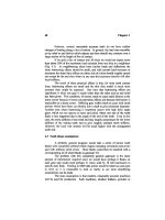
Fig
14.4 Contrast between
tip
relief shape
for
conventional design
and
corresponding
fast
change
at tip for low
contact ratio design.
Low
Contact Ratio Gears
227

14.2
Disadvantages
The
major
advantages
in
root strength associated with large teeth
would
appear
to
give
low
contact ratio gears
a
great advantage
but in
practice
they
are
little used.
The
main
reason
for
this
is
that
it is
difficult
to get a

smooth changeover with
a low
contact ratio
as any
theoretical
tip
relief design
must
occur
in a
very short distance
if
there
is to be low
T.E. Fig. 14.4 shows
Harris maps which contrast
the tip
reliefs
for a
high contact ratio mesh
and a
conventional
mesh.
The
changeover
is
very dependant
on
accuracy
of

profile
generation
and on
having
the
centre distance exact.
This
is not
important
for
very
low
speed gears where
dynamics
can be
ignored.
It is
also
less
important
for
very small gears since
for
small gears
the
manufacturing
errors become much larger
in
relation
to

elastic deflections
and
pitch
and
profile
errors become
sufficiently
large that they dominate
the
meshing.
As the
changeover errors
are
large they dominate
the
T.E. changes
regardless
of the
nominal contact ratio
so
there
is
little noise penalty associated
with
using
a low
contact ratio.
The
main disadvantages
from

strength aspects
lie in the
problems
at
the
ends
of the flanks
where changeover occurs
as
exceptionally high
stresses
are
generated.
As can be
seen
in
Fig. 14.3,
at the
bottom
of the
pinion tooth
the
contact
is
very near
the
base
circle
so the
radius

of
curvature
of the
involute
profile
is
very small.
The
standard Hertzian contact
stress
formulae
for
cylindrical
contacts depend
on the
effective
combined radius
of
curvature
which
in
this
case,
with rack teeth,
is
equal
to the
local pinion curvature.
As
this

drops near
the
base circle
the
contact
stresses
rise
to
about double
the
value
at
the
pitch point.
At
the tip of the
pinion teeth there
is a
different
problem
in
that
the
radius
of
curvature
is
relatively large
so the
Hertzian

stresses
are
below half
those
at the
root
but the
tips
of the
teeth
are
very narrow. There
is
high
friction
with
very slow running gears
so in one
direction
of
rotation there
can be a
high
force,
approaching tangential
in
direction,
attempting
to
shear

off the
tips
of
the
teeth.
The
shear
stresses
across
the
narrow
tip
combined with
the
local
contact
stresses
can
give
failure.
Another problem
can
arise
as the
pinion
tip is
narrow, only allowing
a
small radius
of

curvature
so
manufacturing
or
positioning inaccuracies
may run the
contact onto
the tip
which, with
its
small
radius,
will
give high contact
stresses.
14.3 Curvature Problems
The
small radius
of
curvature
of the
profile
at the
pinion root
was
mentioned
as a
problem
in
stressing.

Our
standard assumption
is
that
the
radius
of
curvature
is
equal
to the
length
of the
tangent
from the
base circle.
In
228
Chapter
14
1.08:
1.06
1.04
1.02
tangent
from
-0.1
position
base
circle

0.98
L
•-
<


1
-—
— -
—
-0.12
-0.1 -0.08 -0.06 -0.04 -0.02
0
Fig
14.5 Expanded view
of
involute near base circle.
the
limit,
if the
working
profile
reaches down
to the
base circle,
the
length
of
the
tangential unwrapping string becomes zero

and
then theoretically
we
have
zero radius
of
curvature
and so
very high contact
stresses.
This does
not
agree with
commonsense
because
if we
look
at the
shape
of an
involute
as it
starts
out from the
base circle,
it
does
not
look
like

a
small
radius
of
curvature.
It
starts
out by
moving almost radially outwards
as
can be
seen
in
Fig. 14.3. with
no
hint
of the
sharp point
we
would expect
with
zero radius
of
curvature. Double-checking
the
mathematics
by
alternative
methods still gives zero
as the

radius
of
curvature.
When mathematics
and
common
sense
do not
agree
it is
usually
(invariably)
the
mathematics that
is
wrong.
In
this
case
the
reason
for the
silly
answer
is
that near
the
base circle
the
centre

of the
radius
of
curvature
(at the
tangent point
to the
base circle)
is
travelling
as
fast
in the
tangential direction
as the
radius
is
reducing.
The net
effect
is
that
the
effective
curvature
is not as
sharp
as
expected. This presents problems when assessing contact
stresses

since
the
effective
radius
of
contact
is
very much higher than
the
theoretical
value.
Various attempts have been made
to
modify
the
involute shape near
the
base
circle
to
avoid
the
theoretical
low
radius problem
but it is
debatable
whether there
is
much point

in
such modification when there
is in
reality
a
Low
Contact Ratio Gears
229
higher radius than expected. Fig. 14.5 shows
the
involute shape down near
the
base circle drawn
out
accurately
and
shows
the
tangent
at the
point
0.1
radian
unwrap
angle. With seven teeth this unwrap angle corresponds
to
only about
one
tenth
of a

base
pitch.
As can be
seen,
there
is no
detectable reduction
in
curvature
for the first
part
of the
involute.
For
highly loaded gears such
as
jacking
rig
gears
there
is an
additional
factor
that
eases
the
local
stresses.
It is
customary

to
design
for the
rack teeth
to
reach
the
plastic state each time they
are
loaded.
The
deformations
involved spread
the
contact patch over
a
large area
and so
reduce
stress
levels greatly.
The
teeth surfaces
deform
permanently
and the
width
of
the
rack teeth increases

but the
rack material
is
relatively
soft
and
does
not
fracture
and
the
required
life
of the
gears
is a
restricted number
of
cycles
so the
gears
are
satisfactory.
14.4 Frequency gains
As
mentioned previously,
a
standard "fix"
for
noise problems

is to
alter
the
number
of
teeth
to
alter
the
excitation
frequency.
This
has
usually
taken
the
form
of
increasing
the
number
of
teeth
to
push
the
tooth
frequency
out
of a

troublesome resonance region. There
is a
stress
penalty associated
with
finer
teeth
as
root
stresses
rise and,
in
general, this approach
will
only
help
if the
tooth
frequencies are
already high,
say
above
1
kHz.
In
general,
reducing
the
size
of the

teeth does
not
reduce
the
T.E.
at
I/tooth
so it is
equally
likely
that noise will rise.
An
alternative that
can be
useful
is
when
the
1/tooth
is
relatively low,
say
below
500 Hz.
Reducing
the
number
of
teeth
will

drive
the frequency
down
to the
region where human hearing becomes much less sensitive
and
this
is
reflected
in the
standard
A
weighting used.
At a
given sound pressure level
reducing
the frequency from 200 Hz to
100
Hz
corresponds
to a
nearly
10
dB
improvement
on the A
weighting scale.
Another advantage
of
reducing

frequency is
that sound
pressure
levels
depend
on
velocity
of
panel vibration
so
that
if the
vibration
is at
constant
amplitude
(as the
T.E. remains constant amplitude)
the frequency
reduction
reduces velocity correspondingly.
Speeds must
be
relatively
low for frequency
reduction
to
help.
The
standard motor speed

of
1450
rpm
will
give about
400 Hz
with
a 19
tooth
pinion
so the
number
of
teeth needs
to be
reduced
to
about
11
to
pull tooth
frequency
down
to the
order
of 200 Hz. If
possible
it is
much quieter
to use the

traditional design
of a 3 or 4 to 1
initial
reduction
by
belt
drive-
then tooth
frequencies are in a
quiet region.
15
Condition
Monitoring
15.1
The
problem
Condition monitoring
of
gears (and
of
bearings) using vibration
is an
area where very large amounts
of
sophisticated electronics
and
computing
mathematics
have been employed

at
great expense
but
with rather limited
effectiveness.
The
objective
is to
give some
form
of
warning
of
trouble
before
it
happens,
not
after
teeth have disappeared. This
may be
simply
to
allow
industrial
machinery
to be
maintained during
the
weekend

before
it
breaks
down
and
stops production
in
mid-week
or,
more critically,
it may be to
give
the
time necessary
for a
helicopter
to
land before
the
rotor jams. Alternative
methods such
as
chemical analysis
of the oil or
debris monitoring
are
sensitive
but
tend
to be too

slow
for
immediate warning.
Originally,
a
couple
of
generations ago, standard
accelerometers
were
fitted
on
bearing housings
and a
meter
indicated
rms
or
power over
the
whole
frequency
range.
An
overall
rise
in
vibration power indicated trouble.
The
first

development
was to
filter
(analog) into octave
or
third octave bands
and
monitor
the
power
in
each band.
The
next stage (once cheap
fast
digital
FFT
routines were available),
was to
carry
out a
full
frequency
analysis, giving
major
lines
at
I/rev, I/tooth, etc.,
and
watch each individual line.

Any
significant
increase
in
amplitude
of any
line indicated trouble
(in
theory).
Some
30
years later
a
paper
by Ray
[1]
summed
up the
state
of the
then current art.
The
vibration signal
was frequency
analysed
but was
also
split into
frequency
bands, possibly six, covering

the
range,
and
each
filtered
band
was
subjected
to a
Kurtosis
analysis. This involved taking
the 4th
order
of
the
variation
of the
vibration signal
from the
mean (zero)
and
normalising
it
by
dividing
by the
square
of the
mean power
in the

signal.
The
resulting non-
dimensional
statistical
ratio would
be
less
than
3 for a
well-behaved random
Gaussian distribution signal
but
would
be
greater than
3 for a
signal which
was
"peaky."
(In
some work
3 is
subtracted
from the
value.)
The
resulting criteria
from frequency
analysis line changes

and filtered
band Kurtosis
figures
were
assessed
to see if
anything
had
changed
"significantly
or if
Kurtosis
was too
high
and if so, red
lights appeared
to
indicate that there
was a
fault.
By the
time
a
warning appeared
it was
often
too
late
and a
considerable number

of
231
232
Chapter
15
false
warnings destroyed operator confidence. Since then there
has
been
considerable
refinement
of the
electronics but,
in
terms
of
fundamentals, little
progress.
It
should perhaps
be
commented that
gears
are not
usually
the
weak
spot
in
gearboxes

and
that commonly
it is
bearings which
fail,
so any
monitoring system must
be
good
at
detecting bearing problems.
The
requirements
for
bearing monitoring
are
surprisingly
different
from
those
of
gear teeth
but
fortunately, monitoring bearings
is,
technically,
a
rather
easier
problem.

15.2
Not
frequency analysis
The
automatic reaction
of a
vibration engineer
is to do a frequency
analysis
of a
signal,
but
though this
may be
useful
for
noise (and
may
tell
you
how
many teeth there
are on the
gear)
it is of
very limited
use for
damage
monitoring. This
is

because
FFT
analysis gives
the
power
in a
spectrum line,
spread over
the
test length
which
is
usually
1
rev.
(a)
ampl
(b)
ampl
(c)
ampl
r\
one
revolution
Fig
15.1 Time
traces:
(a) is for a
single high tooth
and (b) for a

single
low
tooth;
(c) is the
difference
of
either
from the
regular
1/tooth
pattern.
Condition Monitoring
233
Fig.
15.1
(a)
shows
an
idealised signal, predominantly
at
1/tooth
for a
revolution
of a
gear with
an odd
fault
on one
tooth
and

Fig.
12.1(b)
shows
a
similar
odd
fault.
Frequency analysis
of
such signals would show
a
negligible
difference
from the
analysis
of a
gear with regular once
per
tooth
and
some
background
random noise.
In
fact
the
difference
between
the
results

from
either
Fig
15.1
(a) or
Fig
15.
l(b)
and a
regular
waveform
would
be
exactly
the
same
as the frequency
analysis
of the
subtracted signal shown
in
Fig.
15.1(c).
A
small pulse such
as
this,
occuring
for
only

a
short time
in the
revolution would give very small
components spread over
a
wide
frequency
range.
These would
be
completely
lost
in the
background noise
and
random variations present
in any
real system.
We
are
left
with
the
problem that although
we can see a
fault
very
clearly
in the

original time
trace,
simple
frequency
analysis completely hides
the
fault
so we
will
not see
significant variations
in
line amplitudes unless
all
the
teeth
are
damaged. This would
be an
extremely unusual
or
extremely
powerful
fault.
The
same
fundamental
problem occurs with methods based
on
statistical

analysis. Since
a
problem
on 1
tooth
of a 100
tooth gear
may
only
occur
for 1% of the
time
the
power level associated with
the
problem
is
very
low
when spread over
the
whole revolution
so it can
easily disappear into
the
background
noise.
15.3 Averaging
or not
Time averaging

of a
vibration signal
is a
very
useful
and
powerful
method
for
reducing
the
volume
of
information
and
eliminating random noise
and
non-synchronous vibration.
In
general,
it is
useful
for
monitoring
purposes
but
should
be
used with caution
for

some
faults.
If
a
fault
gives
a
perfectly consistent
effect
from
revolution
to
revolution, then averaging
is a
great help.
A
hole
in a
gear tooth surface
due
to
spalling
or
loss
of
part
of a
tooth will,
in
theory, give

a
signal which
is
consistent over many revolutions
and
which
can be
detected
and
analysed
much
more
effectively
if
averaging
at the frequency of
that
shaft
is
being used.
Wear
or
scuffing
are by
their nature inconsistent
and not so
amenable
to
averaging.
A

particular asperity that
is
being
scuffed
away
may be
removed
in
a few
revolutions once
the
surface
has
been torn
up and the
scuffing
may
then move
to
another part
of the
tooth occuring
at a
slightly
different
time
in
the
revolution.
The

effect
of
averaging over
a
large number
of
revolutions will
then
be to
smooth
out the
variations over
a
long period
and to
hide
the
effects.
This leaves
a
problem
in
that,
for
monitoring
cracking,
major
pitting
or
spalling,

we
might wish
to
average over
a
large number
of
revs, perhaps
256.
In
contrast,
for
scuffing,
probably averaging over
8 or 16
revs would
be
234
Chapter
15
more suitable
so
that
we get
some noise reduction
effects
but do not
risk losing
relatively
transient

effects.
A
further
possibility arises
if we are
interested
in
using vibration
monitoring
as a
method
of
detecting dirt
or
debris passing through
the
mesh.
Here
the
vibration pulse
only
occurs once
or
perhaps twice
and we are
interested
in
catching that part
of the
signal that

is not
regular.
The
most
sensitive approach
is to
time-average
the
signal
at
both pinion
and
wheel
frequency
and
subtract
the
averages
from the
original time trace (before
averaging)
to
leave
just
the
intermittent
transient
effects.
An
alternative

is to
high-pass
the
signal
to
remove eccentricities, then
to
average
at
once-per-tooth
frequency
and
deduct
to
remove
the
main part
of the
"regular"
signal, leaving
mainly
transients.
With
the
main regular (low
frequency)
components
removed,
any
short transients should

be
easier
to
detect. This
will
only work
well
if the
once-per-tooth components
are
consistent.
15.4 Damage criteria
Starting
from a
vague
feeling
that damage ought
to
give some sort
of
variation
on a
vibration
or
noise signal does
not
give
a
direct indication
of

what
an
observed change
of
vibration means
in
terms
of
damage.
It is
worthwhile
attempting
to
predict what character
of
signal
the
three standard
types
of
damage might produce
and how
large that signal
may be.
Pitting
is the
most common
and
widespread damage that occurs with
gears

and
although
90% of
pitting stabilises
and is not
threatening
to
gear
life,
it
would
be
helpful
to be
able
to
detect
it. On a
medium-sized gear
a pit may
be 1 mm
diameter.
On a
spur gear tooth with standard
20°
pressure angle
and
100
mm
pitch radius

at
1500
rpm
the
rolling velocity near
the
pitch line
(where
the
pits usually occur)
is 0.1 sin 20° * 50
TT
which
is
roughly
5
m/s.
Assuming
a
working facewidth
of
100
mm and a
mean contact loading
of 280
N/mm
(20
^m
elastic deflection) means that
the

expected change
in
force level
will
be at
most
280 N if
speeds were high enough that
the
gear masses
did not
have
time
to
move. Alternatively,
if the
gears
were rotating
at
very
low
speeds
we
would expect
a
displacement
of 0.2
urn. This,
of
course, assumes that there

is
no
averaging
out of
effects
due to a
thick
oil film.
At
full
speed
we
may,
at
most, expect
a
differential
force
pulse
[as in
Fig.
15.1(c)]
which
was 280 N
high
and 0.2
milliseconds long.
A
half sinusoid
pulse

of
this size
would
produce
a
displacement
of a 14 kg
mass
of the
order
of
less than
1/4 of a
micron amplitude. This hypothetical size
of
displacement
pulse must
be
considered
in
relation
to
normal T.E. excitation
of the
order
of 5
um.
If
there
are

several pitting craters near
the
pitch line
the
situation
becomes
more complicated since
one pit
crater
may
take over
as
another
Condition
Monitoring
235
finishes,
giving
a
relatively steady length
of
line
of
contact
on a
helical gear
and,
hence,
a
steady deflection.

A
further
complication arises with helical
gears
if we
guess
that
there
might
be 20
pits
associated
with each tooth interval since
our
tooth
frequency
might
be 600 Hz
(1500
rpm
and 24
teeth)
and the pit frequency
would
then
be
12
kHz. This high
a frequency
will

be
attenuated
by the
internal dynamics
and
will
have
difficulty
in
travelling
out to the
bearing housing
accelerometers
through
either rolling bearings
or
plain bearings, even
if the
pulses
are
short
enough
not to
overlap
and
give
a
steady
deflection. Both
hydrodynamic

and
rolling types
of
bearing tend
to
reflect
fast
pulses rather than transmitting
them.
The
overall conclusion
is
that
it is
going
to be
extremely
difficult
to
see
vibration
effects
at a
bearing housing
due to
pitting. Part
of the
problem
is
that

the
excitation
is
small compared with normal T.E.
and
part
is
that high
frequencies,
well
above internal system natural
frequencies,
will have very
great
difficulty
in
getting
out to the
bearing housing.
Tooth root cracking
is
potentially
a
very serious
fault
so it is
worthwhile
guessing what
effect
a

cracked tooth would give.
The
main
effect
of
a
large crack along
the
root
of a
tooth would
be to
reduce
the
bending
stiffiiess
of the
tooth
and
reduce
the
load taken
by
that part
of the
tooth.
An
extreme case would
be if the
stiffiiess

was so low
that
the
cracked part
of the
tooth took
no
load
at
all,
as if
that section
of
tooth
had
disappeared.
If
we
take
a
particular condition where
25% of the
axial length
of a
helical tooth
has
"disappeared"
then, with
a
contact ratio

of
1.5, assuming
perfectly
even bedding along
the
total contact line length,
the
remaining
contact line length will
be 5/6 of the
uncracked
length.
T.E.
peak
value
roughly
20%
of
mean
deflection
A
one
revolution
Fig
15.2 Change
in
T.E.
due to
part
of

tooth missing.
236
Chapter
15
Ignoring system dynamics, this
will
give
an
increase
of 20% in the
mean
deflection
and
would increase elastic deflection
from say 20 um to 24
um.
The
effect
of
this
"missing"
tooth section
on
static T.E. under
full
load
will
be as
indicated
in

Fig. 15.2. This
is a
sketch
of the
change
in
T.E. that
would
be
superposed
on the
normal T.E.
There would
be a
gradual run-in
of the
extra
4 um
with
the
rate
depending
on the
exact design
and a
corresponding gradual runout. Since
the
changes
are
smooth there would

not be
very high harmonic components. This
order
of
level
of
change,
4 um,
would
be
detectable
in a
very high precision
gearbox such
as a
helicopter gearbox which
was
heavily loaded.
However,
on a
normal industrial
gearbox,
variations
of
this level
can
be
encountered routinely
from
manufacturing

errors
such
as
pitch errors and,
in
position
in
equipment, there
may be
external transients
as
well
as
system
dynamics
to
mask
any
effects
from the
broken tooth. High speed gearboxes
present
an
additional problem
because
at
6000
rpm
the
tooth

frequency is
already
2.5 kHz and
vibration pulses less than
0.1
milliseconds long
are
unlikely
to be
transmitted
effectively
through
the
bearings
to the
bearing
housings.
Again
the
discouraging conclusion
is
that
it may be
difficult
to
detect
much
change
in the
vibration pattern even with

a
quarter
of a
tooth missing
unless conditions
are
very favourable.
This
conclusion
is
borne
out in
practice
since
it has
been known
for
significant chunks
of
teeth
to be
lost without
any
noticeable external
effects.
The
damage
was
only detected when stripping
down

for
routine maintenance.
The
third main category
of
trouble
is in the
area
of
scuffing
and
wear,
either
due to
breakdown
of the oil
film
or due to
debris
and
dirt
in the
oil.
Metal-to-metal
contact
is
involved
and
either
asperities

on the
mating surfaces
come into contact through
the oil
film
or
welding occurs between
the
surfaces.
The
major problem with this type
of
fault
again lies
in the
very short time scale
involved.
Asperities
are
small, perhaps
20 um
long
and 2 um
high, typically,
so if
there
is a
rolling
or
sliding velocity

of the
order
of 1
m/s
the
pressure
pulse
is
only
20 us
long
and is
typically only
2 N
peak force. This
is too
short
for
standard
accelerometers
to
detect
and
will
not
transmit satisfactorily
through
either rolling bearings
or
plain bearings

to
bearing housings.
These
rather pessimistic estimates give
an
idea
of why
using vibration
to
monitor gear damage
is
difficult,
because
however sophisticated
the
mathematics,
if the
information
is not
originally within
the
vibration trace
it
cannot
be
extracted. Alternatively
if the
information
of
interest

is
dominated
by
synchronous noise
it
cannot
be
separated.
Needless
to
say,
any
suggestion
that
the
damage information
may not be
there
in the
signal early enough
(to be
extracted)
is
highly
controversial with commercial developers
of
monitoring
equipment.
Condition Monitoring
237

The
disturbances
for
pitting
are
essentially
of the
order
of 1% of the
mean
load
and are at too
high
a frequency to
transmit
out
well.
For
root
cracking,
the
disturbances
are
larger,
typically
of the
order
of 5% of the
mean
load

but are
comparable
in
size with commercial errors
and in the
same
frequency
range.
15.5 Line elimination
Since
we are
looking
for
small intermittent changes
in
pattern,
a
different
technique
is
needed.
original
signal
T.E
T.E
difference
"one revolution
Fig
15.3 Line elimination
and

resynthesis
to
detect small changes.
238
Chapter
15
In
section 15.2
it was
commented that
frequency
analysis
would
not
easily show
the
small
differences
between Fig.
15.1
(a) or
15.1(b)
and a
steady
signal, despite
the
visible
difference.
A
technique

to
show
the
difference
is
line
elimination
and
resynthesis.
This
was
mentioned
in
section 9.7, where
the
objective
was to
dispose
of
large lines
but is of
more general
use to
show
occasional changes.
The
example given
in
section
9.7 was of a

small phase change
on one
displaced tooth
but the
same technique
can
show
up
other small changes. Fig.
15.3(a)
shows
a
vibration
trace
for one
(averaged) revolution
of a
gear.
FFT
analysis followed
by
removal
of all
lines
at
1/tooth
and
harmonics subtracts
the
regular signal

in
Fig.
15.3(b)
and
resynthesis
of
what
is
left
(by
inverse Fourier transform) gives
the
signal
in
15.3(c),
showing
a
problem
at the
changeover
from one
tooth
to the
next.
Automatic
analysis
of the
resynthesised
residual signal
can be

attempted using
Kurtosis
(statistical) methods
but
these
can be
unreliable,
for
example
if a
steady sine wave
or
square wave
is
present.
It is
probably simpler
to use the
very
old
fashioned
"crest
factor" which
is the
ratio
of the
peak value
to the
rms
for the

whole rev.
Any
automated method
is
subject
to
errors
so it is
often
worthwhile looking
at the
residual signal since human vision
is
remarkably
effective
at
picking
out
oddities
in a
pattern.
A
more refined version
of
this approach
has
been developed
by Dr.
McFadden
[2].

The
technique
is
similar
but
makes
the
assumption that there
is
a
damaged section restricted
to say
10%
of the
rotation
of the
gear. Which
10%
of the
gear,
is of
course
not
known initially,
so the
analysis uses
the
difference
between
a

previous test
and the
current test
to find a
sector which
may
have
a
problem.
The
approach also adjusts
the
test results
to
allow
for
small
changes
in
speed
or
angular reference position.
The
remaining
90% of
the
rotation
is
analysed
to

derive
the
steady "correct"
frequency
components
of
vibration
and
these components
are
subtracted
from the
vibration
to
leave
the
extra components
associated
with
the
damaged section. Significant extra
components then indicate damage
and
where
it is
around
the
gear.
15.5 Scuffing: Smith shocks
The

previous sections
suggested
that detecting disturbances
of the
order
of 1% in the
presence
of
high background variations
was
extremely
difficult
in
industrial gearboxes.
In
contrast
scuffing
gives asperity contacts
which
generate forces
of the
order
of 2 N
compared with possibly
20,OOON
mean
force
so
should
be

undetectable.
The
difference lies
in the
time
scales
involved
since
root
cracks would
give vibration
at frequencies of the
order
of
tooth
frequency
whereas
scuffing
gives pulses
only
about
20
u.s
long.
Condition
Monitoring
239
at
c
c

o
2
*
4>
0
U
0)
£
.*:
(0
4)
0,
n
u
-50
-100
-150
-200
-250
-300
-350
Tooth
Tooth
Tooth
Tooth
Tooth
Tooth
Tooth
Tooth
Tooth

Tooth
No
No
No
No
No
No
No
No
No
No
1
,***,
2
3
4
5
ilfllrttatJi
JlMrflUfa
HlJIflfl
•
™ri|f
Tl™"™™™[
7
s
l>^
8
>,*^
r
"

1
.

10
50
100
Time
in
minutes
150
-100
-150
-200
-250
-300
150
Time
in
minutes
Fig
15.4
Test
results
from
Smith
shock
investigations
of
scuffing
failure.