Handbook of Corrosion Engineering Episode 1 Part 2 docx

1.3 Kinetic Principles
Thermodynamic principles can help explain a corrosion situation in
terms of the stability of chemical species and reactions associated with
corrosion processes. However, thermodynamic calculations cannot be
used to predict corrosion rates. When two metals are put in contact,
they can produce a voltage, as in a battery or electrochemical cell (see
Galvanic Corrosion in Sec. 5.2.1). The material lower in what has been
called the “galvanic series” will tend to become the anode and corrode,
while the material higher in the series will tend to support a cathodic
reaction. Iron or aluminum, for example, will have a tendency to cor-
rode when connected to graphite or platinum. What the series cannot
predict is the rate at which these metals corrode. Electrode kinetic
principles have to be used to estimate these rates.
1.3.1 Kinetics at equilibrium: the exchange
current concept
The exchange current I
0
is a fundamental characteristic of electrode
behavior that can be defined as the rate of oxidation or reduction at an
equilibrium electrode expressed in terms of current. The term
exchange current, in fact, is a misnomer, since there is no net current
flow. It is merely a convenient way of representing the rates of oxida-
tion and reduction of a given single electrode at equilibrium, when no
loss or gain is experienced by the electrode material. For the corrosion
of iron, Eq. (1.1), for example, this would imply that the exchange cur-
32 Chapter One
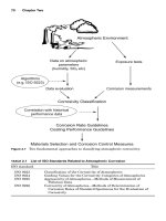
Stresses due to
corrosion product buildup
Voluminous corrosion
products
Cracking and spalling of the concrete cover

Reinforcing steel
Reduced pH levels due to carbonation
Figure 1.15 Graphical representation of the corrosion of reinforcing steel in concrete
leading to cracking and spalling.
0765162_Ch01_Roberge 9/1/99 2:46 Page 32
rent is related to the current in each direction of a reversible reaction,
i.e., an anodic current I
a
representing Eq. (1.7) and a cathodic current
I
c
representing Eq. (1.8).
Fe → Fe
2ϩ
ϩ 2e
Ϫ
(1.7)
Fe ← Fe
2ϩ
ϩ 2e
Ϫ
(1.8)
Since the net current is zero at equilibrium, this implies that the
sum of these two currents is zero, as in Eq. (1.9). Since I
a
is, by con-
vention, always positive, it follows that, when no external voltage or
current is applied to the system, the exchange current is as given by
Eq. (1.10).
I

a
ϩ I
c
ϭ 0 (1.9)
I
a
ϭϪI
c
ϭ I
0
(1.10)
There is no theoretical way of accurately determining the exchange
current for any given system. This must be determined experimental-
ly. For the characterization of electrochemical processes, it is always
preferable to normalize the value of the current by the surface area of
the electrode and use the current density, often expressed as a small i,
i.e., i ϭ I/surface area. The magnitude of exchange current density is
a function of the following main variables:
1. Electrode composition. Exchange current density depends upon
the composition of the electrode and the solution (Table 1.1). For redox
reactions, the exchange current density would depend on the composi-
tion of the electrode supporting an equilibrium reaction (Table 1.2).
Aqueous Corrosion 33
TABLE 1.1 Exchange Current Density (i
0
)
for M
z+
/M Equilibrium in Different Acidified
Solutions (1M)

Electrode Solution log
10
i
0
, A/cm
2
Antimony Chloride Ϫ4.7
Bismuth Chloride Ϫ1.7
Copper Sulfate Ϫ4.4; Ϫ1.7
Iron Sulfate Ϫ8.0; Ϫ8.5
Lead Perchlorate Ϫ3.1
Nickel Sulfate Ϫ8.7; Ϫ6.0
Silver Perchlorate 0.0
Tin Chloride Ϫ2.7
Titanium Perchlorate Ϫ3.0
Titanium Sulfate Ϫ8.7
Zinc Chloride Ϫ3.5; Ϫ0.16
Zinc Perchlorate Ϫ7.5
Zinc Sulfate Ϫ4.5
0765162_Ch01_Roberge 9/1/99 2:46 Page 33
Table 1.3 contains the approximate exchange current density for the
reduction of hydrogen ions on a range of materials. Note that the val-
ue for the exchange current density of hydrogen evolution on platinum
is approximately 10
Ϫ2
A/cm
2
, whereas that on mercury is 10
Ϫ13
A/cm

2
.
2. Surface roughness. Exchange current density is usually
expressed in terms of projected or geometric surface area and depends
upon the surface roughness. The higher exchange current density for
the H
ϩ
/H
2
system equilibrium on platinized platinum (10
Ϫ2
A/cm
2
)
compared to that on bright platinum (10
Ϫ3
A/cm
2
) is a result of the larg-
er specific surface area of the former.
3. Soluble species concentration. The exchange current is also a
complex function of the concentration of both the reactants and the
products involved in the specific reaction described by the exchange
current. This function is particularly dependent on the shape of the
charge transfer barrier ␤ across the electrochemical interface.
34 Chapter One
TABLE 1.2 Exchange Current Density (i
0
) at 25°C for Some Redox Reactions
System Electrode Material Solution log

10
i
0
, A/cm
2
Cr
3ϩ
/Cr
2ϩ
Mercury KCl Ϫ6.0
Ce
4ϩ
/Ce
3ϩ
Platinum H
2
SO
4
Ϫ4.4
Fe
3ϩ
/Fe
2ϩ
Platinum H
2
SO
4
Ϫ2.6
Rhodium H
2

SO
4
Ϫ7.8
Iridium H
2
SO
4
Ϫ2.8
Palladium H
2
SO
4
Ϫ2.2
H
ϩ
/H
2
Gold H
2
SO
4
Ϫ3.6
Lead H
2
SO
4
Ϫ11.3
Mercury H
2
SO

4
Ϫ12.1
Nickel H
2
SO
4
Ϫ5.2
Tungsten H
2
SO
4
Ϫ5.9
O
2
reduction Platinum Perchloric acid Ϫ9.0
Platinum 10%–Rhodium Perchloric acid Ϫ9.0
Rhodium Perchloric acid Ϫ8.2
Iridium Perchloric acid Ϫ10.2
TABLE 1.3 Approximate
Exchange Current Density (i
0
) for
the Hydrogen Oxidation Reaction
on Different Metals at 25°C
Metal log
10
i
0
, A/cm
2

Pb, Hg Ϫ13
Zn Ϫ11
Sn, Al, Be Ϫ10
Ni, Ag, Cu, Cd Ϫ7
Fe, Au, Mo Ϫ6
W, Co, Ta Ϫ5
Pd, Rh Ϫ4
Pt Ϫ2
0765162_Ch01_Roberge 9/1/99 2:46 Page 34
4. Surface impurities. Impurities adsorbed on the electrode sur-
face usually affect its exchange current density. Exchange current den-
sity for the H
ϩ
/H
2
system is markedly reduced by the presence of trace
impurities like arsenic, sulfur, and antimony.
1.3.2 Kinetics under polarization
When two complementary processes such as those illustrated in Fig.
1.1 occur over a single metallic surface, the potential of the material
will no longer be at an equilibrium value. This deviation from equilib-
rium potential is called polarization. Electrodes can also be polarized
by the application of an external voltage or by the spontaneous pro-
duction of a voltage away from equilibrium. The magnitude of polar-
ization is usually measured in terms of overvoltage ␩, which is a
measure of polarization with respect to the equilibrium potential E
eq
of
an electrode. This polarization is said to be either anodic, when the
anodic processes on the electrode are accelerated by changing the spec-

imen potential in the positive (noble) direction, or cathodic, when the
cathodic processes are accelerated by moving the potential in the neg-
ative (active) direction. There are three distinct types of polarization
in any electrochemical cell, the total polarization across an electro-
chemical cell being the summation of the individual elements as
expressed in Eq. (1.11):
␩
total
ϭ␩
act
ϩ␩
conc
ϩ iR (1.11)
where ␩
act
ϭ activation overpotential, a complex function describing
the charge transfer kinetics of the electrochemical
processes. ␩
act
is predominant at small polarization cur-
rents or voltages.
␩
conc
ϭ concentration overpotential, a function describing the
mass transport limitations associated with electrochemi-
cal processes. ␩
conc
is predominant at large polarization
currents or voltages.
iR ϭ ohmic drop. iR follows Ohm’s law and describes the polar-

ization that occurs when a current passes through an
electrolyte or through any other interface, such as surface
film, connectors, etc.
Activation polarization. When some steps in a corrosion reaction con-
trol the rate of charge or electron flow, the reaction is said to be under
activation or charge-transfer control. The kinetics associated with
apparently simple processes rarely occur in a single step. The overall
anodic reaction expressed in Eq. (1.1) would indicate that metal atoms
Aqueous Corrosion 35
0765162_Ch01_Roberge 9/1/99 2:46 Page 35
in the metal lattice are in equilibrium with an aqueous solution contain-
ing Fe
2ϩ
cations. The reality is much more complex, and one would need
to use at least two intermediate species to describe this process, i.e.,
Fe
lattice
→ Fe
ϩ
surface
Fe
ϩ
surface
→ Fe
2ϩ
surface
Fe
2ϩ
surface
→ Fe

2ϩ
solution
In addition, one would have to consider other parallel processes,
such as the hydrolysis of the Fe
2ϩ
cations to produce a precipitate or
some other complex form of iron cations. Similarly, the equilibrium
between protons and hydrogen gas [Eq. (1.2)] can be explained only by
invoking at least three steps, i.e.,
H
ϩ
→ H
ads
H
ads
ϩ H
ads
→ H
2 (molecule)
H
2 (molecule)
→ H
2 (gas)
The anodic and cathodic sides of a reaction can be studied individual-
ly by using some well-established electrochemical methods in which the
response of a system to an applied polarization, current or voltage, is
studied. A general representation of the polarization of an electrode sup-
porting one redox system is given in the Butler-Volmer equation (1.12):
i
reaction

ϭ i
0
Ά
exp
΂
␤
reaction
␩
reaction
΃
Ϫ
exp
΄
Ϫ (1 Ϫ␤
reaction
) ␩
reaction
΅·
(1.12)
where i
reaction
ϭ
anodic or cathodic current
␤
reaction
ϭ charge transfer barrier or symmetry coefficient for the
anodic or cathodic reaction, close to 0.5
␩
reaction
ϭ E

applied
Ϫ E
eq
, i.e., positive for anodic polarization and
negative for cathodic polarization
n ϭ number of participating electrons
R ϭ gas constant
T ϭ absolute temperature
F ϭ Faraday
nF
ᎏ
RT
nF
ᎏ
RT
36 Chapter One
0765162_Ch01_Roberge 9/1/99 2:46 Page 36
When ␩
reaction
is anodic (i.e., positive), the second term in the Butler-
Volmer equation becomes negligible and i
a
can be more simply
expressed by Eq. (1.13) and its logarithm, Eq. (1.14):
i
a
ϭ i
0
΄
exp

΂
␤
a
␩
a
΃΅
(1.13)
␩
a
ϭ b
a
log
10
΂΃
(1.14)
where b
a
is the Tafel coefficient that can be obtained from the slope of
a plot of ␩ against log i, with the intercept yielding a value for i
0
.
b
a
ϭ 2.303 (1.15)
Similarly, when ␩
reaction
is cathodic (i.e., negative), the first term in
the Butler-Volmer equation becomes negligible and i
c
can be more sim-

ply expressed by Eq. (1.16) and its logarithm, Eq. (1.17), with b
c
obtained by plotting ␩ versus log i [Eq. (1.18)]:
i
c
ϭ i
0
Ά
Ϫ exp
΄
Ϫ(1 Ϫ␤
c
) ␩
c
΅·
(1.16)
␩
c
ϭ b
c
log
10
΂΃
(1.17)
b
c
ϭϪ2.303 (1.18)
Concentration polarization. When the cathodic reagent at the corroding
surface is in short supply, the mass transport of this reagent could
become rate controlling. A frequent case of this type of control occurs

when the cathodic processes depend on the reduction of dissolved oxy-
gen. Table 1.4 contains some data related to the solubility of oxygen in
air-saturated water at different temperatures, and Table 1.5 contains
some data on the solubility of oxygen in seawater of different salinity
and chlorinity.
10
Because the rate of the cathodic reaction is proportional to the sur-
face concentration of the reagent, the reaction rate will be limited by a
drop in the surface concentration. For a sufficiently fast charge trans-
fer, the surface concentration will fall to zero, and the corrosion
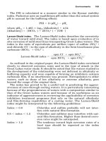
process will be totally controlled by mass transport. As indicated in
Fig. 1.16, mass transport to a surface is governed by three forces: dif-
RT
ᎏ
␤nF
i
c
ᎏ
i
0
nF
ᎏ
RT
RT
ᎏ
␤nF
i
a
ᎏ
i

0
nF
ᎏ
RT
Aqueous Corrosion 37
0765162_Ch01_Roberge 9/1/99 2:46 Page 37
fusion, migration, and convection. In the absence of an electric field,
the migration term is negligible, and the convection force disappears
in stagnant conditions.
For purely diffusion-controlled mass transport, the flux of a species
O to a surface from the bulk is described with Fick’s first law (1.19),
J
O
ϭϪD
O
΂΃
(1.19)
where J
O
ϭ flux of species O, mol и s
Ϫ1
и cm
Ϫ2
D
O
ϭ diffusion coefficient of species O, cm
2
и s
Ϫ1
ϭ concentration gradient of species O across the interface,

mol и cm
Ϫ4
The diffusion coefficient of an ionic species at infinite dilution can be
estimated with the help of the Nernst-Einstein equation (1.20), which
relates D
O
to the conductivity of the species (␭
O
):
␦C
O
ᎏ
␦x
␦C
O
ᎏ
␦x
38 Chapter One
TABLE 1.4 Solubility of Oxygen in Air-Saturated Water
Temperature, °C Volume, cm
3
* Concentration, ppm Concentration (M), ␮mol/L
0 10.2 14.58 455.5
5 8.9 12.72 397.4
10 7.9 11.29 352.8
15 7.0 10.00 312.6
20 6.4 9.15 285.8
25 5.8 8.29 259.0
30 5.3 7.57 236.7
*cm

3
per kg of water at 0°C.
TABLE 1.5 Oxygen Dissolved in Seawater in Equilibrium with a Normal
Atmosphere
Chlorinity,* % 0 5 10 15 20
Salinity,† % 0 9.06 18.08 27.11 36.11
Temperature, °C ppm
0 14.58 13.70 12.78 11.89 11.00
5 12.79 12.02 11.24 10.49 9.74
10 11.32 10.66 10.01 9.37 8.72
15 10.16 9.67 9.02 8.46 7.92
20 9.19 8.70 8.21 7.77 7.23
25 8.39 7.93 7.48 7.04 6.57
30 7.67 7.25 6.80 6.41 5.37
*Chlorinity refers to the total halogen ion content as titrated by the addition of silver
nitrate, expressed in parts per thousand (%).
†Salinity refers to the total proportion of salts in seawater, often estimated empirically as
chlorinity ϫ 1.80655, also expressed in parts per thousand (%).
0765162_Ch01_Roberge 9/1/99 2:46 Page 38
D
O
ϭ (1.20)
where z
O
ϭ the valency of species O
R ϭ gas constant, i.e., 8.314 J и mol
Ϫ1
и K
Ϫ1
T ϭ absolute temperature, K

F ϭ Faraday’s constant, i.e., 96,487 C и mol
Ϫ1
Table 1.6 contains values for D
O
and ␭
O
of some common ions. For
more practical situations, the diffusion coefficient can be approximat-
ed with the help of Eq. (1.21), which relates D
O
to the viscosity of the
solution ␮ and absolute temperature:
D
O
ϭ (1.21)
where A is a constant for the system.
TA
ᎏ
␮
RT␭
O
ᎏ
|z
O
|
2
F
2
Aqueous Corrosion 39
H

+
e
-
H
+
H
+
2e
-
e
-
H
+
Fe
2+
Fe
2+
Charge transfer
Mass transport
activation barrier ( )␣
exchange current density (i )
0
Tafel slope (b)
convection
diffusion
migration
Figure 1.16 Graphical representation of the processes occurring at an electrochemical
interface.
0765162_Ch01_Roberge 9/1/99 2:46 Page 39
TABLE 1.6 Conductivity and Diffusion Coefficients of Selected Ions at Infinite Dilution in Water at 25°C

Cation |z| ␭, S и cm
2
и mol
Ϫ1
D ϫ 10
5
, cm
2
и s
Ϫ1
Anion |z| ␭, S и cm
2
и mol
Ϫ1
D ϫ 10
5
, cm
2
и s
Ϫ1
H
ϩ
1 349.8 9.30 OH
Ϫ
1 197.6 5.25
Li
ϩ
1 38.7 1.03 F
Ϫ
1 55.4 1.47

Na
ϩ
1 50.1 1.33 Cl
Ϫ
1 76.3 2.03
K
ϩ
1 73.5 1.95 NO
3
Ϫ
1 71.4 1.90
Ca
2ϩ
2 119.0 0.79 ClO
4
Ϫ
1 67.3 1.79
Cu
2ϩ
2 107.2 0.71 SO
4
2Ϫ
2 160.0 1.06
Zn
2ϩ
2 105.6 0.70 CO
3
2Ϫ
2 138.6 0.92
O

2
—— 2.26 HSO
4
Ϫ
1 50.0 1.33
H
2
O —— 2.44 HCO
3
Ϫ1
1 41.5 1.11
40
0765162_Ch01_Roberge 9/1/99 2:46 Page 40
The region near the metallic surface where the concentration gra-
dient occurs is also called the diffusion layer ␦. Since the concentra-
tion gradient ␦C
O
/␦x is greatest when the surface concentration of
species O is completely depleted at the surface (i.e., C
O
ϭ 0), it follows
that the cathodic current is limited in that condition, as expressed by
Eq. (1.22):
i
c
ϭ i
L
ϭϪnFD
O
(1.22)

For intermediate cases, ␩
conc
can be evaluated using an expression
[Eq. (1.23)] derived from the Nernst equation:
␩
conc
ϭ log
10
΂
1 Ϫ
΃
(1.23)
where 2.303RT/F ϭ 0.059 V when T ϭ 298.16 K.
Ohmic drop. The ohmic resistance of a cell can be measured with a
milliohmmeter by using a high-frequency signal with a four-point
technique. Table 1.7 lists some typical values of water conductivity.
10
While the ohmic drop is an important parameter to consider when
designing cathodic and anodic protection systems, it can be mini-
mized, when carrying out electrochemical tests, by bringing the refer-
ence electrode into close proximity with the surface being monitored.
For naturally occurring corrosion, the ohmic drop will limit the influ-
ence of an anodic or a cathodic site on adjacent metal areas to a cer-
tain distance depending on the conductivity of the environment. For
naturally occurring corrosion, the anodic and cathodic sites often are
adjacent grains or microconstituents and the distances involved are
very small.
i
ᎏ
i

L
2.303RT
ᎏᎏ
nF
C
O,,
bulk
ᎏ
␦
Aqueous Corrosion 41
TABLE 1.7 Resistivity of Waters
Water ␳, ⍀иcm
Pure water 20,000,000
Distilled water 500,000
Rainwater 20,000
Tap water 1000–5000
River water (brackish) 200
Seawater (coastal) 30
Seawater (open sea) 20–25
0765162_Ch01_Roberge 9/1/99 2:46 Page 41
1.3.3 Graphical presentation of kinetic data
Electrode kinetic data are typically presented in a graphical form
called Evans diagrams, polarization diagrams, or mixed-potential dia-
grams. These diagrams are useful in describing and explaining many
corrosion phenomena. According to the mixed-potential theory under-
lying these diagrams, any electrochemical reaction can be algebraical-
ly divided into separate oxidation and reduction reactions with no net
accumulation of electric charge. In the absence of an externally
applied potential, the oxidation of the metal and the reduction of some
species in solution occur simultaneously at the metal/electrolyte inter-

face. Under these circumstances, the net measurable current is zero
and the corroding metal is charge-neutral, i.e., all electrons produced
by the corrosion of a metal have to be consumed by one or more cathod-
ic processes (e
Ϫ
produced equal e
Ϫ
consumed with no net accumulation
of charge).
It is also important to realize that most textbooks present corrosion
current data as current densities. The main reason for that is simple:
Current density is a direct characteristic of interfacial properties.
Corrosion current density relates directly to the penetration rate of a
metal. If one assumes that a metallic surface plays equivalently the
role of an anode and that of a cathode, one can simply balance the cur-
rent densities and be done with it. In real cases this is not so simple.
The assumption that one surface is equivalently available for both
processes is indeed too simplistic. The occurrence of localized corrosion
is a manifest proof that the anodic surface area can be much smaller
than the cathodic. Additionally, the size of the anodic area is often
inversely related to the severity of corrosion problems: The smaller the
anodic area and the higher the ratio of the cathodic surface S
c
to the
anodic surface S
a
, the more difficult it is to detect the problem.
In order to construct mixed-potential diagrams to model a corrosion
situation, one must first gather (1) the information concerning the
activation overpotential for each process that is potentially involved

and (2) any additional information for processes that could be affected
by concentration overpotential. The following examples of increasing
complexity will illustrate the principles underlying the construction of
mixed-potential diagrams.
The following sections go through the development of detailed equa-
tions and present some examples to illustrate how mixed-potential
models can be developed from first principles.
1. For simple cases in which corrosion processes are purely activation-
controlled
2. For cases in which concentration controls at least one of the corro-
sion processes
42 Chapter One
0765162_Ch01_Roberge 9/1/99 2:46 Page 42
Activation-controlled processes. For purely activation-controlled
processes, each reaction can be described by a straight line on an E
versus log i plot, with positive Tafel slopes for anodic processes and
negative Tafel slopes for cathodic processes. The corrosion anodic
processes are never limited by concentration effects, but they can be
limited by the passivation or formation of a protective film.
Note: Since 1 mA и cm
Ϫ2
corresponds to a penetration rate of 1.2 cm per
year, it is meaningless, in corrosion studies, to consider current densi-
ty values higher than 10 mA и cm
Ϫ2
or 10
Ϫ2
A и cm
Ϫ2
.

The currents for anodic and cathodic reactions can be obtained
with the help of Eqs. (1.14) and (1.17), respectively, which generally
state how the overpotential varies with current, as in the following
equation:
␩ϭb log
10
(I/I
0
) ϭ b log
10
(I) Ϫ b log
10
(I
0
)
where ␩ϭE Ϫ E
eq
E ϭ E
applied
E
eq
ϭ equilibrium or Nernst potential
I
0
ϭ exchange current ϭ i
0
S
i
0
ϭ exchange current density

S ϭ surface area
One normally uses the graphical representation, illustrated in
cases 1 to 3, to determine E
corr
and I
corr
. It is also possible to solve
these problems mathematically, as illustrated in the following trans-
formations.
The applied potential is
E ϭ E
eq
ϩ b log
10
(I) Ϫ b log
10
(I
0
)
and the applied current can then be written as
log
10
(I) ϭϩlog
10
(I
o
) ϭϩlog
10
(I
0

)
or
I ϭ 10
[(E Ϫ E
eq
)/b ϩ log
10
(I
0
)]
at E
corr
,
I
a
ϭ I
c
and E
a
ϭ E
c
ϭ E
corr
and hence
E Ϫ E
eq
ᎏ
b
␩
ᎏ

b
Aqueous Corrosion 43
0765162_Ch01_Roberge 9/1/99 2:46 Page 43
ϩ log
10
(I
0, a
) ϭϩlog
10
(I
0, c
)
or
b
c
(E
corr
Ϫ E
eq, a
) ϩ b
c
b
a
log
10
(I
0, a
) ϭ b
a
(E

corr
Ϫ E
eq, c
) ϩ b
c
b
a
log
10
(I
0, c
)
and
b
c
E
corr
Ϫ b
a
E
corr
ϭ b
c
E
eq, a
Ϫ b
a
E
eq, c
ϩ b

c
b
a
[log
10
(I
0, c
) Ϫ log
10
(I
0, a
) ]
finally
E
corr
ϭϩ
One can obtain I
corr
by substituting E
corr
in one of the previous
expressions, i.e.,
E
corr
ϭ E
eq, a
ϩ b
a
log
10

(I
corr
) Ϫ b log
10
(I
0, a
)
or
b
a
log
10
(I
corr
) ϭ E
corr
Ϫ E
eq, a
ϩ b log
10
(I
0, a
)
and
log
10
(I
corr
) ϭ
First case: iron in a deaerated acid solution at 25

°
C, pH ϭ 0.
Anodic reaction
Surface area ϭ 1 cm
2
Fe → Fe
2ϩ
ϩ 2e
Ϫ
E
0
ϭ Ϫ0.44 V versus SHE
For a corroding metal, one can assume that E
eq
ϭ E
0
.
i
0
ϭ 10
Ϫ6
A и cm
Ϫ2
I
0
ϭ 1 ϫ 10
Ϫ6
A
b
a

ϭ 0.120 V/decade
E
corr
Ϫ E
eq, a
ϩ b log
10
(I
0, a
)
ᎏᎏᎏᎏ
b
a
b
c
b
a
[log
10
(I
0, c
) Ϫ log
10
(I
0, a
) ]
ᎏᎏᎏᎏ
b
c
Ϫ b

a
b
c
E
eq, a
Ϫ b
a
E
eq, c
ᎏᎏ
b
c
Ϫ b
a
(E
corr
Ϫ E
eq, c
)
ᎏᎏ
b
c
E
corr
Ϫ E
eq, a
ᎏᎏ
b
a
44 Chapter One

0765162_Ch01_Roberge 9/1/99 2:46 Page 44
Cathodic reaction
Surface area ϭ 1 cm
2
2H
ϩ
ϩ2e
Ϫ
→ H
2
E
0
ϭ 0.0 V versus SHE
E
eq
ϭ E
0
ϩ 0.059 log
10
a
H
ϩ
ϭ 0.0 ϩ 0 ϭ 0.0 V versus SHE
i
0
ϭ 10
Ϫ6
A и cm
Ϫ2
I

0
ϭ 1 ϫ 10
Ϫ6
A
b
c
ϭ Ϫ0.120 V/decade
The mixed-potential diagram of this system is shown in Fig. 1.17,
and the resultant polarization plot of the system is shown in Fig. 1.18.
Second case: zinc in a deaerated acid solution at 25°C, pH ϭ 0.
Anodic reaction
Zn → Zn
2ϩ
ϩ 2e
Ϫ
E
0
ϭ Ϫ0.763 V versus SHE
Aqueous Corrosion 45
-0.6
-0.5
-0.4
-0.3
-0.2
-0.1
0
0.1
0.2
Potential (V vs SHE)
Log (I(A))

2H
+
+ 2e
-

→
H
2
Fe
→
Fe
2+
+ 2e
-
E
corr
& I
corr
-8 -7 -6 -5 -4 -3 -2
Figure 1.17 The iron mixed-potential diagram at 25°C and pH 0.
0765162_Ch01_Roberge 9/1/99 2:46 Page 45
For a corroding metal, one can assume that E
eq
ϭ E
0
.
i
0
ϭ 10
Ϫ7

A и cm
Ϫ2
b
a
ϭ 0.120 V/decade
Cathodic reaction
2H
ϩ
ϩ 2e
Ϫ
→ H
2
E
0
ϭ 0.0 V versus SHE
E
eq
ϭ E
0
ϩ 0.059 log a
H
ϩ
ϭ 0.0 ϩ 0 ϭ 0.0 V versus SHE
i
0
ϭ 10
Ϫ10
A и cm
Ϫ2
b

a
ϭ Ϫ0.120 V/decade
The mixed-potential diagram of this system is shown in Fig. 1.19,
and the resultant polarization plot of the system is shown in Fig. 1.20.
Third case: iron in a deaerated neutral solution at 25°C, pH ϭ 5.
46 Chapter One
-5.5 -5 -4.5 -4 -3.5 -3 -2.5 -2
-0.4
-0.3
-0.2
-0.1
0
Potential (V vs SHE)
Log (I(A))
2H
+
+ 2e
-

→
H
2
Fe
→
Fe
2+
+ 2 e
-
E
corr

& I
corr
Figure 1.18 The polarization curve corresponding to iron in a pH 0 solution at 25°C
(Fig. 1.17).
0765162_Ch01_Roberge 9/1/99 2:46 Page 46
Anodic reaction
Surface area ϭ 1 cm
2
Fe → Fe
2ϩ
ϩ 2e
Ϫ
E
0
ϭ Ϫ0.44 V versus SHE
For a corroding metal, one can assume that E
eq
ϭ E
0
.
i
0
ϭ 10
Ϫ6
A и cm
Ϫ2
I
0
ϭ 1 ϫ 10
Ϫ6

A
b
a
ϭ 0.120 V/decade
Cathodic reaction
Surface area ϭ 1 cm
2
2H
ϩ
ϩ 2e
Ϫ
→ H
2
E
eq
ϭ E
0
ϩ 0.059 log
10
a
H
ϩ
ϭ 0.0 Ϫ 0.059 ϫ (Ϫ5) ϭ Ϫ0.295 V versus SHE
i
0
ϭ 10
Ϫ6
A и cm
Ϫ2
I

0
ϭ 1ϫ10
Ϫ6
A
b
c
ϭ Ϫ0.120 V/decade
Aqueous Corrosion 47
-12 -11 -10 -9 -8 -7 -6 -5 -4 -3 -2
-1
-0.8
-0.6
-0.4
-0.2
0
0.2
Potential (V vs SHE)
Log (I(A))
2H
+
+ 2e
-

→
→ →
→
H
2
Zn
→

→ →
→
Zn
2+
+ 2e
-
E
corr
& I
corr
Figure 1.19 The zinc mixed-potential diagram at 25°C and pH 0.
0765162_Ch01_Roberge 9/1/99 2:46 Page 47
-7 -6 -5 -4 -3 -2 -1
-1
-0.9
-0.8
-0.7
-0.6
-0.5
-0.4
-0.3
-0.2
Potential (V vs SHE)
Log (I(A))
2H
+
+ 2e
-

→

→ →
→
H
2
Zn
→
→ →
→
Zn
2+
+ 2e
-
E
corr
& I
corr
Figure 1.20 The polarization curve corresponding to zinc in a pH 0 solution at 25°C
(Fig. 1.19).
-0.6
-0.5
-0.4
-0.3
-0.2
-0.1
0
Potential (V vs SHE)
Log (I(A))
2H
+
+ 2e

-

→
H
2
Fe
→
Fe
2+
+ 2e
-
E
corr
& I
corr
-8 -7 -6 -5 -4 -3 -2
Figure 1.21 The iron mixed-potential diagram at 25°C and pH 5.
48
0765162_Ch01_Roberge 9/1/99 2:46 Page 48
The mixed-potential diagram of this system is shown in Fig. 1.21,
and the resultant polarization plot of the system is shown in Fig. 1.22.
Concentration-controlled processes. When concentration control is
added to a process, it simply adds to the polarization, as in the follow-
ing equation:.
␩
tot
ϭ␩
act
ϩ␩
conc

We know that, for purely activation-controlled systems, the current
can be derived from the voltage with the following expression:
I ϭ 10
[(E Ϫ E
eq
)/b ϩ log
10
(I
0
)]
In order to simplify the expression of the current in the presence of
concentration effects suppose that
A ϭ 10
[ (E Ϫ E
eq
)/b ϩ log
10
(I
0
)]
␩
tot
ϭ E Ϫ E
eq
ϭ␩
act
ϩ␩
conc
and
I ϭ I

1
и A/(I
1
ϩ A)
Aqueous Corrosion 49
-0.5
-0.45
-0.4
-0.35
-0.3
-0.25
-0.2
Potential (V vs SHE)
Log (I(A))
2H
+
+ 2e
-

→
H
2
Fe
→
Fe
2+
+ 2e
-
E
corr

& I
corr
-5.8 -5.6 -5.4 -5.2 -5 -4.8 -4.6 -4.4 -4.2 -4-6
Figure 1.22 The polarization curve corresponding to iron in a pH 5 solution at 25°C
(Fig. 1.21).
0765162_Ch01_Roberge 9/1/99 2:46 Page 49
where I
1
is the limiting current of the cathodic process.
Fourth case: iron in an aerated neutral solution at 25°C, pH ϭ 5,
I
1
ϭ 10
Ϫ4
A.
Anodic reaction
Surface area ϭ 1 cm
2
Fe → Fe
2ϩ
ϩ 2e
Ϫ
For a corroding metal, one can assume that E
eq
ϭ E
0
.
i
0
ϭ 10

Ϫ6
A и cm
Ϫ2
I
0
ϭ 1 ϫ 10
Ϫ6
A
b
a
ϭ 0.120 V/decade
Cathodic reactions
Surface area ϭ 1 cm
2
2H
ϩ
ϩ 2e
Ϫ
→ H
2
E
eq
ϭ E
0
ϩ 0.059 log
10
a
H
ϩ
ϭ 0.0 ϩ 0.059 ϫ (Ϫ5) ϭ Ϫ0.295 V versus SHE

i
0
ϭ 10
Ϫ6
A и cm
Ϫ2
I
0
ϭ 1 ϫ 10
Ϫ6
A
b
c
ϭ Ϫ0.120 V/decade
O
2
ϩ 4H
ϩ
ϩ 4e
Ϫ
→ 2H
2
O
E
0
ϭ 1.229 V versus SHE
E
eq
ϭ E
0

ϩ 0.059 log
10
a
H
ϩ
ϩ (0.059/4) log
10
(pO
2
)
Supposing pO
2
ϭ 0.2,
E
eq
ϭ 1.229 Ϫ 0.059 ϫ (Ϫ5) ϩ 0.0148 ϫ (Ϫ0.699) ϭ 0.9237 V versus SHE
i
0
ϭ 10
Ϫ7
A и cm
Ϫ2
I
0
ϭ 1 ϫ 10
Ϫ7
A
b
c
ϭ Ϫ0.120 V/decade

i
1
ϭ I
1
ϭ 10
Ϫ4
A
The mixed-potential diagram of this system is shown in Fig. 1.23,
and the resultant polarization plot of the system is shown in Fig. 1.24.
Fifth case: iron in an aerated neutral solution at 25°C, pH ϭ 2, I
1
ϭ
10
Ϫ4.5
A.
Surface area ϭ 1 cm
2
50 Chapter One
0765162_Ch01_Roberge 9/1/99 2:46 Page 50
-8 -7 -6 -5 -4 -3 -2
-0.8
-0.6
-0.4
-0.2
0
0.2
0.4
0.6
0.8
1

Potential (V vs SHE)
Log (I(A))
2H
+
+ 2e
-
→
H
2
Fe
→
Fe
2+
+ 2e
-
E
corr
& I
corr
O
2
+ 4H
+
+ 4e
-
→
2H
2
O
Figure 1.23 The iron mixed-potential diagram at 25°C and pH 5 in an aerated solution

with a limiting current of 10
Ϫ4
A for the reduction of oxygen.
-6 -5.5 -5 -4.5 -4 -3.5 -3 -2.5 -2
-0.7
-0.6
-0.5
-0.4
-0.3
-0.2
-0.1
0
Potential (V vs SHE)
Log (I(A))
2H
+
+ 2e
-

→
H
2
Fe
→
Fe
2+
+ 2e
-
E
corr

& I
corr
O
2
+ 4H
+
+ 4e
-
→ 2
H
2
O
Figure 1.24 The polarization curve corresponding to iron in a pH 5 solution at 25°C in an
aerated solution with a limiting current of 10
Ϫ4
A for the reduction of oxygen (Fig. 1.23).
51
0765162_Ch01_Roberge 9/1/99 2:46 Page 51
-8 -7 -6 -5 -4 -3 -2
-0.8
-0.6
-0.4
-0.2
0
0.2
0.4
0.6
0.8
1
Potential (V vs SHE)

Log (I(A))
2H
+
+ 2e
-
→
H
2
Fe
→
Fe
2+
+ 2e
-
E
corr
& I
corr
O
2
+ 4H
+
+ 4e
-
→ 2
H
2
O
Figure 1.25 The iron mixed-potential diagram at 25°C and pH 2 in an aerated solution
with a limiting current of 10

Ϫ4.5
A for the reduction of oxygen.
-6 -5.5 -5 -4.5 -4 -3.5 -3 -2.5 -2
-0.6
-0.5
-0.4
-0.3
-0.2
-0.1
0
Potential (V vs SHE)
Log (I(A))
2H
+
+ 2e
-
→
H
2
Fe
→
Fe
2+
+ 2e
-
E
corr
& I
corr
O

2
+ 4H
+
+ 4e
-
→ 2
H
2
O
Figure 1.26 The polarization curve corresponding to iron in a pH 2 solution at 25°C in an
aerated solution with a limiting current of 10
Ϫ4.5
A for the reduction of oxygen (Fig. 1.25).
52
0765162_Ch01_Roberge 9/1/99 2:46 Page 52
-8 -7 -6 -5 -4 -3 -2
-0.8
-0.6
-0.4
-0.2
0
0.2
0.4
0.6
0.8
1
Potential (V vs SHE)
Log (I(A))
2H
+

+ 2e
-
→
H
2
Fe
→
Fe
2+
+ 2e
-
E
corr
& I
corr
O
2
+ 4H
+
+ 4e
-
→ 2
H
2
O
Figure 1.27 The iron mixed-potential diagram at 25°C and pH 2 in an aerated solution
with a limiting current of 10
Ϫ5
A for the reduction of oxygen.
-6 -5.5 -5 -4.5 -4 -3.5 -3 -2.5 -2

-0.5
-0.4
-0.3
-0.2
-0.1
0
Potential (V vs SHE)
Log (I(A))
2H
+
+ 2e
-
→
H
2
Fe
→
Fe
2+
+ 2e
-
E
corr
& I
corr
O
2
+ 4H
+
+ 4e

-
→ 2
H
2
O
Figure 1.28 The polarization curve corresponding to iron in a pH 2 solution at 25°C in an
aerated solution with a limiting current of 10
Ϫ5
A for the reduction of oxygen (Fig. 1.27).
53
0765162_Ch01_Roberge 9/1/99 2:46 Page 53
The only differences from the previous case are that (1) the pH has
become more acidic and (2) the limiting current of the cathodic reac-
tion has decreased to 10
Ϫ4.5
A.
2H
ϩ
ϩ 2e
Ϫ
→ H
2
E
eq
ϭ E
0
ϩ 0.059 log
10
a
H

ϩ
ϭ 0.0 ϩ 0.059 ϫ (Ϫ2) ϭ Ϫ0.118 V versus SHE
The mixed-potential diagram of this system is shown in Fig. 1.25,
and the resultant polarization plot of the system is shown in Fig. 1.26.
Sixth case: iron in an aerated neutral solution at 25°C, pH ϭ 2, I
1
ϭ 10
Ϫ5
A.
Surface area ϭ 1 cm
2
The only difference from the previous case is that the limiting cur-
rent of the cathodic reaction has decreased to 10
Ϫ5
A. The mixed-poten-
tial diagram of this system is shown in Fig. 1.27, and the resultant
polarization plot of the system is shown in Fig. 1.28.
References
1. Pourbaix, M., Atlas of Electrochemical Equilibria in Aqueous Solutions, Houston,
Tex., NACE International, 1974.
2. Staehle, R. W., Understanding “Situation-Dependent Strength”: A Fundamental
Objective in Assessing the History of Stress Corrosion Cracking, in Environment-
Induced Cracking of Metals, Houston, Tex., NACE International, 1989, pp. 561–612.
3. Pourbaix, M. J. N., Lectures on Electrochemical Corrosion, New York, Plenum Press,
1973.
4. Guthrie, J., A History of Marine Engineering, London, Hutchinson of London, 1971.
5. Flanagan, G. T. H., Feed Water Systems and Treatment, London, Stanford Maritime
London, 1978.
6. Jones, D. R. H., Materials Failure Analysis: Case Studies and Design Implications,
Headington Hill Hall, U.K., Pergamon Press, 1993.

7. Ruggeri, R. T., and Beck, T. R., An Analysis of Mass Transfer in Filiform Corrosion,
Corrosion 39:452–465 (1983).
8. Slabaugh, W. H., DeJager, W., Hoover, S. E., et al., Filiform Corrosion of Aluminum,
Journal of Paint Technology 44:76–83 (1972).
9. ASTM, Standard Test Method for Half-Cell Potentials of Uncoated Reinforcing Steel
in Concrete, in Annual Book of ASTM Standards, Philadelphia, American Society
for Testing and Materials, 1997.
10. Shreir, L. L., Jarman R. A., and Burstein, G. T., Corrosion Control, Oxford, U.K.,
Butterworth Heinemann, 1994.
54 Chapter One
0765162_Ch01_Roberge 9/1/99 2:46 Page 54
13
Aqueous Corrosion
1.1 Introduction 13
1.2 Applications of Potential-pH Diagrams 16
1.2.1 Corrosion of steel in water at elevated temperatures 17
1.2.2 Filiform corrosion 26
1.2.3 Corrosion of reinforcing steel in concrete 29
1.3 Kinetic Principles 32
1.3.1 Kinetics at equilibrium: the exchange current concept 32
1.3.2 Kinetics under polarization 35
1.3.3 Graphical presentation of kinetic data 42
References 54
1.1 Introduction
One of the key factors in any corrosion situation is the environment.
The definition and characteristics of this variable can be quite com-
plex. One can use thermodynamics, e.g., Pourbaix or E-pH diagrams,
to evaluate the theoretical activity of a given metal or alloy provided
the chemical makeup of the environment is known. But for practical
situations, it is important to realize that the environment is a vari-

able that can change with time and conditions. It is also important to
realize that the environment that actually affects a metal corresponds
to the microenvironmental conditions that this metal really “sees,”
i.e., the local environment at the surface of the metal. It is indeed the
reactivity of this local environment that will determine the real cor-
rosion damage. Thus, an experiment that investigates only the nomi-
nal environmental condition without consideration of local effects
such as flow, pH cells, deposits, and galvanic effects is useless for life-
time prediction.
Chapter
1
0765162_Ch01_Roberge 9/1/99 2:46 Page 13
In our societies, water is used for a wide variety of purposes, from
supporting life as potable water to performing a multitude of industri-
al tasks such as heat exchange and waste transport. The impact of
water on the integrity of materials is thus an important aspect of sys-
tem management. Since steels and other iron-based alloys are the
metallic materials most commonly exposed to water, aqueous corrosion
will be discussed with a special focus on the reactions of iron (Fe) with
water (H
2
O). Metal ions go into solution at anodic areas in an amount
chemically equivalent to the reaction at cathodic areas (Fig. 1.1). In
the cases of iron-based alloys, the following reaction usually takes
place at anodic areas:
Fe → Fe
2ϩ
ϩ 2e
Ϫ
(1.1)

This reaction is rapid in most media, as shown by the lack of pro-
nounced polarization when iron is made an anode employing an exter-
nal current. When iron corrodes, the rate is usually controlled by the
14 Chapter One
H
+
2e
-
H
+
Fe
2+
Figure 1.1 Simple model describ-
ing the electrochemical nature of
corrosion processes.
0765162_Ch01_Roberge 9/1/99 2:46 Page 14