Handbook of Corrosion Engineering Episode 1 Part 5 potx

The PSI is calculated in a manner similar to the Ryznar stability
index. Puckorius uses an equilibrium pH rather than the actual system
pH to account for the buffering effects:
PSI ϭ 2 (pH
eq
) Ϫ pH
s
where pH
eq
ϭ 1.465 ϫ log
10
[Alkalinity] ϩ 4.54
[Alkalinity] ϭ [HCO
3
Ϫ
] ϩ 2[CO
3
2Ϫ
] ϩ [OH
Ϫ
]
Larson-Skold index. The Larson-Skold index describes the corrosivity
of water toward mild steel. The index is based upon evaluation of in
situ corrosion of mild steel lines transporting Great Lakes waters. The
index is the ratio of equivalents per million (epm) of sulfate (SO
4
2Ϫ
)
and chloride (Cl
Ϫ
) to the epm of alkalinity in the form bicarbonate plus

carbonate (HCO
3
Ϫ
ϩ CO
3
2Ϫ
).
Larson-Skold index ϭ
As outlined in the original paper, the Larson-Skold index correlated
closely to observed corrosion rates and to the type of attack in the
Great Lakes water study. It should be noted that the waters studied in
the development of the relationship were not deficient in alkalinity or
buffering capacity and were capable of forming an inhibitory calcium
carbonate film, if no interference was present. Extrapolation to other
waters, such as those of low alkalinity or extreme alkalinity, goes
beyond the range of the original data.
The index has proved to be a useful tool in predicting the aggres-
siveness of once-through cooling waters. It is particularly interesting
because of the preponderance of waters with a composition similar to
that of the Great Lakes waters and because of its usefulness as an
indicator of aggressiveness in reviewing the applicability of corrosion
inhibition treatment programs that rely on the natural alkalinity
and film-forming capabilities of a cooling water. The Larson-Skold
index might be interpreted by the following guidelines:
Index Ͻ 0.8 Chlorides and sulfate probably will not inter-
fere with natural film formation.
0.8 Ͻ index Ͻ 1.2 Chlorides and sulfates may interfere with nat-
ural film formation. Higher than desired corro-
sion rates might be anticipated.
Index Ͼ 1.2 The tendency toward high corrosion rates of a

local type should be expected as the index
increases.
epm Cl
Ϫ
ϩ epm SO
4
2Ϫ
ᎏᎏᎏᎏ
epm HCO
3
Ϫ
ϩ epm CO
3
2Ϫ
Environments 109
0765162_Ch02_Roberge 9/1/99 4:01 Page 109
Stiff-Davis index. The Stiff-Davis index attempts to overcome the
shortcomings of the Langelier index with respect to waters with high
total dissolved solids and the impact of “common ion” effects on the
driving force for scale formation. Like the LSI, the Stiff-Davis index
has its basis in the concept of saturation level. The solubility product
used to predict the pH at saturation (pH
s
) for a water is empirically
modified in the Stiff-Davis index. The Stiff-Davis index will predict
that a water is less scale forming than the LSI calculated for the same
water chemistry and conditions. The deviation between the indices
increases with ionic strength. Interpretation of the index is by the
same scale as for the Langelier saturation index.
Oddo-Tomson index. The Oddo-Tomson index accounts for the impact of

pressure and partial pressure of CO
2
on the pH of water and on the sol-
ubility of calcium carbonate. This empirical model also incorporates cor-
rections for the presence of two or three phases (water, gas, and oil).
Interpretation of the index is by the same scale as for the LSI and Stiff-
Davis indices.
Momentary excess (precipitation to equilibrium). The momentary excess
index describes the quantity of scalant that would have to precipitate
instantaneously to bring water to equilibrium. In the case of calcium
carbonate,
K
spc
ϭ [Ca
2ϩ
] [CO
3
2Ϫ
]
If water is supersaturated, then
[Ca
2ϩ
] [CO
3
2Ϫ
] ӷK
spc
Precipitation to equilibrium assumes that one mole of calcium ions
will precipitate for every mole of carbonate ions that precipitates. On
this basis, the quantity of precipitate required to restore water to equi-

librium can be estimated with the following equation:
[Ca
2ϩ
Ϫ X] [CO
3
2Ϫ
Ϫ X] ϭ K
spc
where X is the quantity of precipitate required to reach equilibrium.
X will be a small value when either calcium is high and carbonate low,
or carbonate is high and calcium low. It will increase to a maximum
when equal parts of calcium and carbonate are present. As a result,
these calculations will provide vastly different values for waters with
the same saturation level. Although the original momentary excess
index was applied only to calcium carbonate scale, the index can be
extended to other scale-forming species. In the case of sulfate, momen-
tary excess is calculated by solving for X in the relationship
110 Chapter Two
0765162_Ch02_Roberge 9/1/99 4:02 Page 110
[Ca
2ϩ
Ϫ X] [SO
4
2Ϫ
Ϫ X] ϭ K
spc
The solution becomes more complex for tricalcium phosphate:
[Ca
2ϩ
Ϫ 3X]

3
[PO
4
3Ϫ
Ϫ 2X]
2
ϭ K
spc
While this index provides a quantitative indicator of scale poten-
tial and has been used to correlate scale formation in a kinetic mod-
el, the index does not account for two critical factors: First, the pH
can often change as precipitates form, and second, the index does not
account for changes in driving force as the reactant levels decrease
because of precipitation. The index is simply an indicator of the
capacity of water to scale, and can be compared to the buffer capaci-
ty of a water.
Interpreting the indices. Most of the indices discussed previously
describe the tendency of a water to form or dissolve a particular scale.
These indices are derived from the concept of saturation. For example,
saturation level for any of the scalants discussed is described as the
ratio of a compound’s observed ion-activity product to the ion-activity
product expected if the water were at equilibrium K
sp
. The following
general guidelines can be applied to interpreting the degree of super-
saturation:
1. If the saturation level is less than 1.0, a water is undersaturated
with respect to the scalant under study. The water will tend to dis-
solve, rather than form, scale of the type for which the index was
calculated. As the saturation level decreases and approaches 0.0,

the probability of forming this scale in a finite period of time also
approaches 0.
2. A water in contact with a solid form of the scale will tend to dissolve
or precipitate the compound until an IAP/K
sp
ratio of 1.0 is
achieved. This will occur if the water is left undisturbed for an infi-
nite period of time under the same conditions. A water with a satu-
ration level of 1.0 is at equilibrium with the solid phase. It will not
tend to dissolve or precipitate the scale.
3. As the saturation level (IAP/K
sp
) increases above 1.0, the tenden-
cy to precipitate the compound increases. Most waters can carry
a moderate level of supersaturation before precipitation occurs,
and most cooling systems can carry a small degree of supersatu-
ration. The degree of supersaturation acceptable for a system
varies with parameters such as residence time, the order of the
scale reaction, and the amount of solid phase (scale) present in
the system.
Environments 111
0765162_Ch02_Roberge 9/1/99 4:02 Page 111
2.2.4 Ion association model
The saturation indices discussed previously can be calculated based
upon total analytical values for all possible reactants. Ions in water,
however, do not tend to exist totally as free ions.
24
Calcium, for example,
may be paired with sulfate, bicarbonate, carbonate, phosphate, and oth-
er species. Bound ions are not readily available for scale formation. This

binding, or reduced availability of the reactants, decreases the effective
ion-activity product for a saturation-level calculation. Early indices such
as the LSI are based upon total analytical values rather than free
species primarily because of the intense calculation requirements for
determining the distribution of species in a water. Speciation of a water
requires numerous computer iterations for the following:
25
■
The verification of electroneutrality via a cation-anion balance, and
balancing with an appropriate ion (e.g., sodium or potassium for
cation-deficient waters; sulfate, chloride, or nitrate for anion-defi-
cient waters).
■
Estimating ionic strength; calculating and correcting activity coef-
ficients and dissociation constants for temperature; correcting
alkalinity for noncarbonate alkalinity.
■
Iteratively calculating the distribution of species in the water from
dissociation constants. A partial listing of these ion pairs is given in
Table 2.13.
■
Verification of mass balance and adjustment of ion concentrations to
agree with analytical values.
■
Repeating the process until corrections are insignificant.
■
Calculating saturation levels based upon the free concentrations of
ions estimated using the ion association model (ion pairing).
The ion association model has been used by major water treatment
companies since the early 1970s. The use of ion pairing to estimate the

concentrations of free species overcomes several of the major shortcom-
ings of traditional indices. While indices such as the LSI can correct
activity coefficients for ionic strength based upon the total dissolved
solids, they typically do not account for common ion effects. Common
ion effects increase the apparent solubility of a compound by reducing
the concentration of available reactants. A common example is sulfate
reducing the available calcium in a water and increasing the apparent
solubility of calcium carbonate. The use of indices which do not account
for ion pairing can be misleading when comparing waters in which the
TDS is composed of ions which pair with the reactants and of ions
which have less interaction with them.
112 Chapter Two
0765162_Ch02_Roberge 9/1/99 4:02 Page 112
The ion association model provides a rigorous calculation of the free
ion concentrations based upon the solution of the simultaneous non-
linear equations generated by the relevant equilibria.
26
A simplified
method for estimating the effect of ion interaction and ion pairing is
sometimes used instead of the more rigorous and direct solution of the
equilibria.
27
Pitzer coefficients estimate the impact of ion association
upon free ion concentrations using an empirical force fit of laboratory
data.
28
This method has the advantage of providing a much less calcu-
lation-intensive direct solution. It has the disadvantages of being
based upon typical water compositions and ion ratios, and of unpre-
dictability when extrapolated beyond the range of the original data.

The use of Pitzer coefficients is not recommended when a full ion asso-
ciation model is available.
When indices are used to establish operating limits such as maxi-
mum concentration ratio or maximum pH, the differences between
indices calculated using ion pairing can have some serious economic
significance. For example, experience on a system with high-TDS water
may be translated to a system operating with a lower-TDS water. The
high indices that were found acceptable in the high-TDS water may be
Environments 113
TABLE 2.13 Examples of Ion Pairs Used to Estimate Free Ion Concentrations
Aluminum
[Aluminum] ϭ [Al
3ϩ
] ϩ [Al(OH)
2ϩ
] ϩ [Al(OH)
2
ϩ
] ϩ [Al(OH)
4
Ϫ
] ϩ [AlF
2ϩ
] ϩ [AlF
2
ϩ
] ϩ
[AlF
3
] ϩ [AlF

4
Ϫ
] ϩ [AlSO
4
ϩ
] ϩ [Al(SO
4
)
2
Ϫ
]
Barium
[Barium] ϭ [Ba
2ϩ
] ϩ [BaSO
4
] ϩ [BaHCO
3
ϩ
] ϩ [BaCO
3
] ϩ [Ba(OH)
ϩ
]
Calcium
[Calcium] ϭ [Ca
2ϩ
] ϩ [CaSO
4
] ϩ [CaHCO

3
ϩ
] ϩ [CaCO
3
] ϩ [Ca(OH)
ϩ
] ϩ [CaHPO
4
] ϩ
[CaPO
4
Ϫ
] ϩ [CaH
2
PO
4
ϩ
]
Iron
[Iron] ϭ [Fe
2ϩ
] ϩ [Fe
3ϩ
] ϩ [Fe(OH)
ϩ
] ϩ [Fe(OH)
2ϩ
] ϩ [Fe(OH)
3
Ϫ

] ϩ [FeHPO
4
ϩ
] ϩ
[FeHPO
4
] ϩ [FeCl
2ϩ
] ϩ [FeCl
2
ϩ
] ϩ [FeCl
3
] ϩ [FeSO
4
] ϩ [FeSO
4
ϩ
] ϩ
[FeH
2
PO
4
ϩ
] ϩ [Fe(OH)
2
ϩ
] ϩ [Fe(OH)
3
] ϩ [Fe(OH)

4
Ϫ
] ϩ [Fe(OH)
2
] ϩ
[FeH
2
PO
4
2ϩ
]
Magnesium
[Magnesium] ϭ [Mg
2ϩ
] ϩ [MgSO
4
] ϩ [MgHCO
3
ϩ
] ϩ [MgCO
3
] ϩ [Mg(OH)
ϩ
] ϩ
[MgHPO
4
] ϩ [MgPO
4
Ϫ
] ϩ [MgH

2
PO
4
ϩ
] ϩ [MgF
ϩ
]
Potassium
[Potassium] ϭ [K
ϩ
] ϩ [KSO
4
Ϫ
] ϩ [KHPO
4
Ϫ
] ϩ [KCl]
Sodium
[Sodium] ϭ [Na
ϩ
] ϩ [NaSO
4
Ϫ
] ϩ [Na
2
SO
4
] ϩ [NaHCO
3
] ϩ [NaCO

3
Ϫ
] ϩ [Na
2
CO
3
] ϩ
[NaCl] ϩ [NaHPO
4
Ϫ
]
Strontium
[Strontium] ϭ [Sr
2ϩ
] 1 [SrSO
4
] 1 [SrHCO
3
ϩ
] ϩ [SrCO
3
] ϩ [Sr(OH)
ϩ
]
0765162_Ch02_Roberge 9/1/99 4:02 Page 113
unrealistic when translated to a water where ion pairing is less signif-
icant in reducing the apparent driving force for scale formation. Table
2.14 summarizes the impact of TDS upon LSI when it is calculated
using total analytical values for calcium and alkalinity, and when it is
calculated using the free calcium and carbonate concentrations deter-

mined with an ion association model.
Indices based upon ion association models provide a common denom-
inator for comparing results between systems. For example, calcite
saturation level calculated using free calcium and carbonate concen-
trations has been used successfully as the basis for developing models
which describe the minimum effective scale inhibitor dosage that will
maintain clean heat-transfer surfaces.
29
The following cases illustrate
some practical usage of the ion association model.
Optimizing storage conditions for low-level nuclear waste. Storage costs
for low-level nuclear wastes are based upon volume. Storage is therefore
most cost-effective when the aqueous-based wastes are concentrated to
occupy the minimum volume. Precipitation is not desirable because it
can turn a low-level waste into a high-level waste, which is much more
costly to store. Precipitation can also foul heat-transfer equipment used
in the concentration process. The ion association model approach has
been used at the Oak Ridge National Laboratory to predict the optimum
conditions for long-term storage.
30
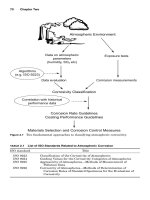
Optimum conditions involve the
parameters of maximum concentration, pH, and temperature. Figures
2.17 and 2.18, respectively, depict a profile of the degree of supersatura-
tion for silica and for magnesium hydroxide as a function of pH and tem-
perature. It can be seen that amorphous silica deposition may present a
problem when the pH falls below approximately 10, and that magne-
sium hydroxide or brucite deposition is predicted when the pH rises
above approximately 11. Based upon this preliminary run, a pH range
of 10 to 11 was recommended for storage and concentration. Other
potential precipitants can be screened using the ion association model to

provide an overall evaluation of a wastewater prior to concentration.
114 Chapter Two
TABLE 2.14 Impact of Ion Pairing on the Langelier Scaling Index (LSI)
LSI
Water Low TDS High TDS TDS impact on LSI
High chloride
No pairing 2.25 1.89 Ϫ0.36
With pairing 1.98 1.58 Ϫ0.40
High sulfate
No pairing 2.24 1.81 Ϫ0.43
With pairing 1.93 1.07 Ϫ0.86
0765162_Ch02_Roberge 9/1/99 4:02 Page 114
Limiting halite deposition in a wet high-temperature gas well. There are
several fields in the Netherlands that produce hydrocarbon gas asso-
ciated with very high TDS connate waters. Classical oilfield scale
problems (e.g., calcium carbonate, barium sulfate, and calcium sul-
fate) are minimal in these fields. Halite (NaCl), however, can be pre-
cipitated to such an extent that production is lost in hours. As a
result, a bottom-hole fluid sample is retrieved from all new wells.
Unstable components are “fixed” immediately after sampling, and pH
is determined under pressure. A full ionic and physical analysis is also
carried out in the laboratory.
The analyses were run through an ion association model computer
program to determine the susceptibility of the brine to halite (and other
scale) precipitation. If a halite precipitation problem was predicted, the
ion association model was run in a “mixing” mode to determine if mixing
the connate water with boiler feedwater would prevent the problem. This
Environments 115
25
34

43
53
62
71
80
13
12
11
10
9
8
7
0
2
4
6
8
10
12
14
16
Saturation Level
Temperature
pH
Figure 2.17 Amorphous silica saturation in low-level nuclear wastewater as a function
of pH and temperature (WaterCycle).
0765162_Ch02_Roberge 9/1/99 4:02 Page 115
approach has been used successfully to control salt deposition in the well
with the composition outlined in Table 2.15. The ion association model
evaluation of the bottom-hole chemistry indicated that the water was

slightly supersaturated with sodium chloride under the bottom-hole con-
ditions of pressure and temperature. As the fluids cooled in the well bore,
the production of copious amounts of halite was predicted.
The ion association model predicted that the connate water would
require a minimum dilution with boiler feedwater of 15 percent to pre-
vent halite precipitation (Fig. 2.19). The model also predicted that over-
injection of dilution water would promote barite (barium sulfate)
formation (Fig. 2.20). Although the well produced H
2
S at a concentra-
tion of 50 mg/L, the program did not predict the formation of iron sul-
fide because of the combination of low pH and high temperature. Boiler
feedwater was injected into the bottom of the well using the downhole
116 Chapter Two
25
34
43
53
62
71
80
13
12
11
10
9
8
7
0
5000

10000
15000
20000
25000
30000
35000
40000
45000
Saturation Level
Temperature
pH
Figure 2.18 Brucite saturation in low-level nuclear wastewater as a function of pH and
temperature.
0765162_Ch02_Roberge 9/1/99 4:02 Page 116
injection valve normally used for corrosion inhibitor injection. Injection
of dilution water at a rate of 25 to 30 percent has allowed the well to
produce successfully since start-up. Barite and iron sulfide precipita-
tion have not been observed, and plugging with salt has not occurred.
Identifying acceptable operating range for ozonated cooling systems. It
has been well established that ozone is an efficient microbiological con-
trol agent in open recirculating cooling-water systems (cooling towers).
It has also been reported that commonly encountered scales have not
been observed in ozonated cooling systems under conditions where
scale would otherwise be expected. The water chemistry of 13 ozonat-
ed cooling systems was evaluated using an ion association model. Each
system was treated solely with ozone on a continuous basis at the rate
of 0.05 to 0.2 mg/L based upon recirculating water flow rates.
31
Environments 117
25

42
58
75
92
108
125
100
83
67
50
33
17
0
0
0.5
1
1.5
2
2.5
Degree of Saturation
Temperature
% Injection
Figure 2.19 Degree of saturation of halite in a hot gas well as a function of temperature
and reinjected boiler water (DownHole SAT).
0765162_Ch02_Roberge 9/1/99 4:02 Page 117
The saturation levels for common cooling-water scales were calcu-
lated, including calcium carbonate, calcium sulfate, amorphous silica,
and magnesium hydroxide. Brucite saturation levels were included
because of the potential for magnesium silicate formation as a result
of the adsorption of silica upon precipitating magnesium hydroxide.

Each system was evaluated by
31
■
Estimating the concentration ratio of the systems by comparing
recirculating water chemistry to makeup water chemistry.
■
Calculating the theoretical concentration of recirculating water
chemistry based upon makeup water analysis and the apparent, cal-
culated concentration ratio from step 1.
■
Comparing the theoretical and observed ion concentrations to deter-
mine precipitation of major species.
■
Calculating the saturation level for major species based upon both
the theoretical and the observed recirculating water chemistry.
■
Comparing differences between the theoretical and actual chem-
istry to the observed cleanliness of the cooling systems and heat
exchangers with respect to heat transfer surface scale buildup,
scale formation in valves and on non–heat-transfer surfaces, and
precipitate buildup in the tower fill and basin.
118 Chapter Two
TABLE 2.15 Hot Gas Well Water Analysis
Bottom hole connate Boiler feedwater
Temperature, °C 121 70
Pressure, bars 350 1
pH, site 4.26 9.10
Density, kg/m
3
1.300 1.000

TDS, mgиL
Ϫ1
369,960 Ͻ20
Dissolved CO
2
, mgиL
Ϫ1
223 Ͻ1
H
2
S (gas phase), mgиL
Ϫ1
50 0
H
2
S (aqueous phase), mgиL
Ϫ1
Ͻ0.5 0
Bicarbonate, mgиL
Ϫ1
16 5.0
Chloride, mgиL
Ϫ1
228,485 0
Sulfate, mgиL
Ϫ1
320 0
Phosphate, mgиL
Ϫ1
Ͻ10

Borate, mgиL
Ϫ1
175 0
Organic acids ϽC
6
, mgиL
Ϫ1
12 Ͻ5
Sodium, mgиL
Ϫ1
104,780 Ͻ1
Potassium, mgиL
Ϫ1
1,600 Ͻ1
Calcium, mgиL
Ϫ1
30,853 Ͻ1
Magnesium, mgиL
Ϫ1
2,910 Ͻ1
Barium, mgиL
Ϫ1
120 Ͻ1
Strontium, mgиL
Ϫ1
1,164 Ͻ1
Total iron, mgиL
Ϫ1
38.0 Ͻ0.01
Lead, mgиL

Ϫ1
5.1 Ͻ0.01
Zinc, mgиL
Ϫ1
3.6 Ͻ0.01
0765162_Ch02_Roberge 9/1/99 4:02 Page 118
Three categories of systems were encountered:
31
■
Category 1. The theoretical chemistry of the concentrated water
was not scale-forming (i.e., undersaturated).
■
Category 2. The concentrated recirculating water would have a
moderate to high calcium carbonate scale–forming tendency. Water
chemistry observed in these systems is similar to that in systems run
successfully using traditional scale inhibitors such as phosphonates.
■
Category 3. These systems demonstrated an extraordinarily high
scale potential for at least calcium carbonate and brucite. These sys-
tems operated with a recirculating water chemistry similar to that
of a softener rather than of a cooling system. The Category 3 water
chemistry was above the maximum saturation level for calcium car-
bonate where traditional inhibitors such as phosphonates are able to
inhibit scale formation.
Environments 119
25
42
58
75
92

108
125
100
83
67
50
33
17
0
0
0.5
1
1.5
2
2.5
3
3.5
Degree of Saturation
Temperature
% Injection
Figure 2.20 Degree of saturation of barite in a hot gas well as a function of temperature
and reinjected boiler water.
0765162_Ch02_Roberge 9/1/99 4:02 Page 119
TABLE 2.16 Theoretical vs. Actual Recirculating Water Chemistry
System Calcium Magnesium Silica
(Category)
T* A† ⌬‡T* A† ⌬‡ T* A† ⌬‡ System cleanliness
1 (1) 56 43 13 28 36 Ϫ84052Ϫ12 No scale observed
2 (2) 80 60 20 88 38 50 24 20 4 Basin buildup
3 (2) 238 288 Ϫ50 483 168 315 38 31 7 Heavy scale

4 (2) 288 180 108 216 223 Ϫ7 66 48 18 Valve scale
5 (3) 392 245 147 238 320 Ϫ82 112 101 11 Condenser tube scale
6 (3) 803 163 640 495 607 Ϫ112 162 143 19 No scale observed
7 (3) 1464 200 1264 549 135 414 112 101 11 No scale observed
8 (3) 800 168 632 480 78 402 280 78 202 No scale observed
9 (3) 775 95 680 496 78 418 186 60 126 No scale observed
10 (3) 3904 270 3634 3172 508 2664 3050 95 2995 Slight valve scale
11 (3) 4170 188 3982 308 303 5 126 126 0 No scale observed
12 (3) 3660 800 2860 2623 2972 Ϫ349 6100 138 5962 No scale observed
13 (3) 7930 68 7862 610 20 590 1952 85 1867 No scale observed
*T ϭ theoretical (ppm).
†A ϭ actual (ppm).
‡⌬ϭdifference (ppm).
120
0765162_Ch02_Roberge 9/1/99 4:02 Page 120
TABLE 2.17 Theoretical vs. Actual Recirculating Water Saturation Level
System
Calcite Brucite Silica
(Category) T* A† T* A† T* A† Observation
1 (1) 0.03 0.02 Ͻ0.001 Ͻ0.001 0.20 0.25 No scale observed
2 (2) 49 5.4 0.82 0.02 0.06 0.09 Basin buildup
3 (2) 89 611 2.4 0.12 0.10 0.12 Heavy scale
4 (2) 106 50 1.3 0.55 0.13 0.16 Valve scale
5 (3) 240 72 3.0 0.46 0.21 0.35 Condenser tube scale
6 (3) 540 51 5.3 0.73 0.35 0.49 No scale observed
7 (3) 598 28 10 0.17 0.40 0.52 No scale observed
8 (3) 794 26 53 0.06 0.10 0.33 No scale observed
9 (3) 809 6.5 10 Ͻ0.01 0.22 0.27 No scale observed
10 (3) 1198 62 7.4 0.36 0.31 0.35 Slight valve scale
11 (3) 1670 74 4.6 0.36 0.22 0.44 No scale observed

12 (3) 3420 37 254 0.59 1.31 0.55 No scale observed
13 (3) 7634 65 7.6 0.14 1.74 0.10 No scale observed
*T ϭ theoretical (ppm).
†A ϭ actual (ppm).
121
0765162_Ch02_Roberge 9/1/99 4:02 Page 121
Table 2.16 outlines the theoretical versus actual water chemistry for
the 13 systems evaluated. Saturation levels for the theoretical and
actual recirculating water chemistries are presented in Table 2.17. A
comparison of the predicted chemistries to observed system cleanli-
ness revealed the following:
31
■
Category 1 (recirculating water chemistry undersaturated). The sys-
tems did not show any scale formation.
■
Category 2 (conventional alkaline cooling system control range).
Scale formation was observed in eight of the nine Category 2 sys-
tems evaluated.
■
Category 3 (cooling tower as a softener). Deposit formation on heat-
transfer surfaces was not observed in most of these systems.
The study revealed that calcium carbonate (calcite) scale formed
most readily on heat-transfer surfaces in systems operating in a cal-
cite saturation level range of 20 to 150, the typical range for chemical-
ly treated cooling water. At much higher saturation levels, in excess of
1000, calcite precipitated in the bulk water. Because of the over-
whelming high surface area of the precipitating crystals relative to the
metal surface in the system, continuing precipitation leads to growth
on crystals in the bulk water rather than on heat-transfer surfaces.

The presence of ozone in cooling systems does not appear to influence
calcite precipitation and/or scale formation.
31
Optimizing calcium phosphate scale inhibitor dosage in a high-TDS cooling
system.
A major manufacturer of polymers for calcium phosphate
scale control in cooling systems has developed laboratory data on the
minimum effective scale inhibitor (copolymer) dosage required to pre-
vent calcium phosphate deposition over a broad range of calcium and
phosphate concentrations, and a range of pH and temperatures. The
data were developed using static tests, but have been observed to cor-
relate well with the dosage requirements for the copolymer in operat-
ing cooling systems. The data were developed using test waters with
relatively low levels of dissolved solids. Recommendations from the
data were typically made as a function of calcium concentration, phos-
phate concentration, and pH. This database was used to project the
treatment requirements for a utility cooling system that used geother-
mal brine for makeup water. An extremely high dosage (30 to 35 mg/L)
was recommended based upon the laboratory data.
25
It was believed that much lower dosages would be required in the
actual cooling system because of the reduced availability of calcium
anticipated in the high-TDS recirculating water. As a result, it was
believed that a model based upon dosage as a function of the ion asso-
ciation model saturation level for tricalcium phosphate would be more
122 Chapter Two
0765162_Ch02_Roberge 9/1/99 4:02 Page 122
appropriate, and accurate, than a simple lookup table of dosage ver-
sus pH and analytical values for calcium and phosphate. Tricalcium
phosphate saturation levels were calculated for each of the laborato-

ry data points. Regression analysis was used to develop a model for
dosage as a function of saturation level and temperature.
The model was used to predict the minimum effective dosage for the
system with the makeup and recirculating water chemistry found in
Table 2.18. A dosage in the range of 10 to 11 mg/L was predicted, rather
than the 30 ppm derived from the lookup tables. A dosage minimization
study was conducted to determine the minimum effective dosage. The
system was initially treated with the copolymer at a dosage of 30 mg/L
in the recirculating water. The dosage was decreased until deposition
was observed. Failure was noted when the recirculating water concen-
tration dropped below 10 mg/L, validating the ion association–based
dosage model.
2.2.5 Software Systems
Some software systems are available for water treatment personnel.
The products combine the calculation sophistication of university-
based mainframe programs with a practical, commonsense engineer-
ing approach to evaluating and solving water treatment problems.
Color-coded graphics in combination with 3-D representation can be
quite useful in visualizing water treatment problems over a user-
defined probable dynamic operating range. Graphics reduce advanced
physical chemistry concepts and profiles to a level where even laypeo-
ple can understand the impact of changing parameters such as pH,
Environments 123
TABLE 2.18 Calcium Phosphate Inhibitor Dosage Optimization Example
Water analysis at 6.2 cycles Deposition potential indicators
Cations Saturation level
Calcium (as CaCO
3
) 1339 Calcite 38.8
Magnesium (as CaCO

3
) 496 Aragonite 32.9
Sodium (as Na) 1240 Silica 0.4
Anions Tricalcium phosphate 1074
Chloride (as Cl) 620 Anhydrite 1.3
Sulfate (as SO
4
) 3384 Gypsum 1.7
Bicarbonate (as HCO
3
) 294 Fluorite 0.0
Carbonate (as CO
3
) 36 Brucite Ͻ0.1
Silica (as SiO
2
) 62 Simple indices
Parameters Langelier 1.99
pH 8.40 Ryznar 4.41
Temperature, °C 36.7 Practical 4.20
Half-life, h 72 Larson-Skold 0.39
Recommended Treatment
100% active copolymer, mg/L 10.53
0765162_Ch02_Roberge 9/1/99 4:02 Page 123
temperature, or concentration. These products serve niche water
treatment markets, including the cooling-water and oilfield markets.
An ion association model engine forms the basis for the sophisticated
predictions of scale, corrosion, and inhibitor optimization provided by
these software systems.
Scaling of cooling water. Watercycle is a computer-based system that

allows a water treatment chemist to evaluate the scale potential for
common scalants over the range of water chemistry, temperature, and
pH anticipated in an operational cooling system.
32
This computer sys-
tem, which was developed to allow water treaters to readily evaluate the
scale potential for common scalants over the broadest of operating
ranges without the necessity for tedious manual calculations, has been
used to generate the analyses presented in this section.
Even when scaling indices can be calculated, they often offer con-
flicting results that can easily cloud the interpretation of what they
are foretelling. The program can be applied to long- as well as short-
residence-time systems. The computer system uses the mean salt
activities for estimating ion-activity coefficients based upon tempera-
ture and ionic strength.
24
The use of ion pairing expands the useful-
ness of calculated saturation levels. The system can assist the cooling
tower operator or water treaters in establishing control limits based on
concentration ratio (cycles of concentration), pH, and temperature
profiles. The program can be used to
■
Develop an overall profile of scale potential for common cooling-
system scalants over the entire range of critical operating parame-
ters anticipated.
■
Evaluate the scale potential of an open recirculating cooling system
versus concentration ratio as an aid in establishing control limits.
■
Evaluate the benefits of pH control with respect to scale potential

and to estimate acid requirements.
■
Review these indicators as water quality changes or environmental
constraints force operation with reduced water quality and
increased scale potential.
■
Learn about the interaction of water chemistry and operating condi-
tions (pH, temperature) by using the program as a system simulator.
Many cooling-water evaluations assume that the cooling system is
static. Indices for scale potential are calculated at the “harshest” con-
ditions for the foulant under study. What-if scenario modeling provides
one of the greatest benefits from using Watercycle. The “what-if scenario”
modules allow one to
124 Chapter Two
0765162_Ch02_Roberge 9/1/99 4:02 Page 124
■
Visualize what will happen to the scale potential and corrosivity of a
cooling water as operating parameters and water chemistry change.
■
Evaluate the current cooling water over the entire range of operat-
ing parameters.
■
Predict water scaling behavior for use in evaluating new cooling sys-
tems, and as an aid in establishing control ranges and operating
parameters.
In the case of calcium carbonate scale, indices are typically calculat-
ed at the highest expected temperature and highest expected pH—the
conditions under which calcium carbonate is least soluble. In the case
of silica, the opposite conditions are used. Amorphous silica has its
lowest solubility at the lowest temperature and lowest pH encoun-

tered. Indices calculated under these conditions would be acceptable in
many cases. Unfortunately, cooling systems are not static. The
foulants silica and tricalcium phosphate are used as examples to
demonstrate the use of operating range profiles in developing an in-
depth evaluation of scale potential and the impact of loss of control.
Silica. Guidelines for the upper silica operating limits have been well
defined in water treatment practice, and have evolved with the treatment
programs. In the days of acid chromate cooling-system treatment, an
upper limit of 150 ppm silica as SiO
2
was common. The limit increased to
180 ppm with the advent of alkaline treatments and pH control limits up
to 9.0. Silica control levels approaching or exceeding 200 ppm as SiO
2
have been reported for the current high-pH, high-alkalinity all-organic
treatment programs where pH is allowed to equilibrate at 9.0 or higher.
26
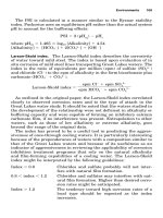
The evolution of silica control limits can be readily understood by
reviewing the silica solubility profile. As depicted in Fig. 2.21, solubility
of amorphous silica increases with increasing pH. Silica solubility also
increases with increasing temperature. In the pH range of 6.0 to 8.0 and
temperature range of 20 to 30°C, cooling water will be saturated with
amorphous silica when the concentration reaches 100 ppm (20°C) or 135
ppm (30°C) as SiO
2
. These concentrations correspond to a saturation
level of 1.0. The traditional silica limit for this pH range has been 150
ppm as SiO
2
. As outlined in Table 2.19, a limit of 150 ppm would corre-

spond roughly to a saturation level of 1.4 at 20°C and 1.1 at 30°C.
At the upper end of the cooling-water pH range (9.0), silica solubili-
ty increases to 115 ppm (20°C) and 140 ppm (30°C). A control limit of
180 ppm would correspond to saturation levels of 1.5 and 1.3, respec-
tively. In systems where concentration ratio is limited by silica solu-
bility, it is recommended that the concentration ratio limit be
reestablished seasonally based on amorphous silica saturation level or
whenever significant temperature changes occur.
26
Environments 125
0765162_Ch02_Roberge 9/1/99 4:02 Page 125
Calcium phosphate. Neutral phosphate programs can benefit from satu-
ration-level profiles for tricalcium phosphate. Treatment programs
using orthophosphate as a corrosion inhibitor must operate in a nar-
row pH range in order to achieve satisfactory corrosion inhibition
without catastrophic calcium phosphate deposition occurring.
Operating-range profiles for tricalcium phosphate can assist the water
treatment chemist in establishing limits for pH, concentration ratio,
and orthophosphate in the recirculating water. Such profiles are also
useful in showing operators the impact of loss of pH control, chemical
overfeed, or overconcentration.
Scaling of deep well water. DownHole SAT is another specialized com-
puter program that allows a water treatment specialist to evaluate the
126 Chapter Two
20
26
32
38
44
50

56
7
7.6
8.4
8.6
8.9
0
50
100
150
200
250
300
350
Soluble silica (mg/l)
Temperature
pH
Figure 2.21 Solubility of amorphous silica as a function of temperature and pH.
TABLE 2.19 Silica Limits for Three Treatment Schemes
Low pH (6.0) Moderate pH (7.6) High pH (8.9)
Temperature (°C) 20 30 20 30 20 30
Silica level (ppm) 130 150 150 150 Ͼ180 Ͼ180
Saturation level limit 1.2 1.1 1.4 1.1 1.5 1.3
0765162_Ch02_Roberge 9/1/99 4:02 Page 126
scale potential for common scalants over a broad range of water chem-
istry parameters, such as temperature, pressure, pH, and pCO
2
.
33
As

with the previous computer system, “what-if scenario” modules pro-
vide an easy way to visualize what could happen to the scale potential
and corrosivity of a water as environmental parameters and water
chemistry change. The what-if scenarios also allow evaluating the
impact of bringing a water to the surface, or finding the safe ratios for
mixing waters under varying conditions. The scenarios can provide a
predictor for use in anticipating problems in new or proposed wells.
The following indices and the scaling behavior of the solid species
shown in Table 2.20 are all calculated by DownHole SAT.
■
Stiff-Davis
■
Oddo-Tomson
■
Ryznar
■
Puckorius
■
Larson-Skold
Convenience groups. Three “convenience groups” have been pro-
grammed into the computer system to allow multiple graph selection
for common groups:
■
The common foulants group includes calcite, barite, witherite, and
anhydrite saturation levels.
■
The common indices group includes the Langelier, Stiff-Davis, Oddo-
Tomson, and Ryznar indices.
Environments 127
TABLE 2.20 Scales Modeled by DownHole SAT

Scale Formula
Calcite CaCO
3
Aragonite CaCO
3
Witherite BaCO
3
Magnesite MgCO
3
Siderite FeCO
3
Barite BaSO
4
Anhydrite CaSO
4
Gypsum CaSO
4
и2H
2
O
Celestite SrSO
4
Fluorite CaF
2
Amorphous iron Fe(OH)
3
Amorphous silica SiO
2
Brucite Mg(OH)
2

Strengite FePO
4
и2H
2
O
Tricalcium phosphate Ca
3
(PO
4
)
2
Hydroxyapatite Ca
5
(PO
4
)
3
(OH)
Thenardite Na
2
SO
4
Halite NaCl
Iron sulfide FeS
0765162_Ch02_Roberge 9/1/99 4:02 Page 127
■
The calcium carbonate group includes calcite saturation level, the
Langelier saturation index, the Stiff-Davis index, and the Oddo-
Tomson index.
Dosages for scale inhibitors should be applied as a function of a driving

force for scale formation and growth (e.g., calcite saturation level), tem-
perature as it affects reaction rates, pH as it affects the dissociation
state of the inhibitor, and time. A version of the computer program
allows the development of mathematical models for the minimum effec-
tive scale inhibitor dosage as a function of these parameters: driving
force, temperature, pH, and time.
Mathematical models. Mathematical models for an inhibitor are devel-
oped by the program using multiple regression. The goodness of fit for
the data can be presented in table and graphical format. Models are
discussed by parameter. The basic parameter to which scale inhibitor
dosages have been correlated historically is the driving force for crys-
tal formation and crystal growth. Early models attempted to develop
models based upon the Langelier saturation index or the Ryznar sta-
bility index. Most water treaters are in agreement that dosage
requirements increase with the driving force for scale formation.
Calcite saturation level provides an excellent driving force for calcium
carbonate scale inhibitor models, gypsum saturation level for calcium
sulfate in the cooling-water temperature range, and tricalcium phos-
phate saturation level for calcium phosphate scale prevention. The
momentary excess indices can also be used effectively to model dosage
requirements.
A second critical factor in determining an effective dosage or devel-
oping a model for an inhibitor is time. Time is the residence time of
scale-forming species in the system you wish to treat. The time factor
for scale inhibition can be as short as 4 to 10 s in a utility condenser
system, or extend into days for cooling towers. In high-saturation-level
systems, the induction period can be very short. In systems where
water is barely supersaturated, the induction time can approach infin-
ity. Scale inhibitors have been observed to extend the induction time
before scale formation or growth on existing scale substrate occurs.

34
Inhibitors extend the time before scale will form in a system by
interfering with the kinetics of crystal formation and growth. Rate
decreases as inhibitor dosages increase. Additional parameters include
temperature, as it affects the rate of crystal formation and/or growth.
Dosage changes with temperature can be modeled with a simple
Arrhenius relationship. pH is an important parameter to include in
these models when an inhibitor can exist in two or more forms within
the pH range of use, and one of the forms is much more active as a
128 Chapter Two
0765162_Ch02_Roberge 9/1/99 4:02 Page 128
scale inhibitor than the other(s). pH can also affect the type of scale
that forms (e.g., tricalcium phosphate versus hydroxylapatite).
2.3 Seawater
2.3.1 Introduction
Seawater systems are used by many industries, such as shipping, off-
shore oil and gas production, power plants, and coastal industrial plants.
The main use of seawater is for cooling purposes, but it is also used for
firefighting, oilfield water injection, and desalination plants. The corro-
sion problems in these systems have been well studied over many years,
but despite published information on materials behavior in seawater,
failures still occur. Most of the elements that can be found on earth are
present in seawater, at least in trace amounts. However, 11 of the con-
stituents account for 99.95 percent of the total solutes, as indicated in
Table 2.21, with chloride ions being by far the largest constituent.
The concentration of dissolved materials in the sea varies greatly
with location and time because rivers dilute seawater, rain, or melting
ice, and seawater can be concentrated by evaporation. The most impor-
tant properties of seawater are
35

■
Remarkably constant ratios of the concentrations of the major con-
stituents worldwide
■
High salt concentration, mainly sodium chloride
■
High electrical conductivity
■
Relatively high and constant pH
■
Buffering capacity
■
Solubility for gases, of which oxygen and carbon dioxide in particu-
lar are of importance in the context of corrosion
■
The presence of a myriad of organic compounds
■
The existence of biological life, to be further distinguished as micro-
fouling (e.g., bacteria, slime) and macrofouling (e.g., seaweed, mus-
sels, barnacles, and many kinds of animals or fish)
Some of these factors are interrelated and depend on physical, chem-
ical, and biological variables, such as depth, temperature, intensity of
light, and the availability of nutrients. The main numerical specifica-
tion of seawater is its salinity.
Salinity. Salinity was defined, in 1902, as the total amount of solid mate-
rial (in grams) contained in one kilogram of seawater when all halides
have been replaced by the equivalent of chloride, when all the carbonate
Environments 129
0765162_Ch02_Roberge 9/1/99 4:02 Page 129
scale inhibitor than the other(s). pH can also affect the type of scale

that forms (e.g., tricalcium phosphate versus hydroxylapatite).
2.3 Seawater
2.3.1 Introduction
Seawater systems are used by many industries, such as shipping, off-
shore oil and gas production, power plants, and coastal industrial plants.
The main use of seawater is for cooling purposes, but it is also used for
firefighting, oilfield water injection, and desalination plants. The corro-
sion problems in these systems have been well studied over many years,
but despite published information on materials behavior in seawater,
failures still occur. Most of the elements that can be found on earth are
present in seawater, at least in trace amounts. However, 11 of the con-
stituents account for 99.95 percent of the total solutes, as indicated in
Table 2.21, with chloride ions being by far the largest constituent.
The concentration of dissolved materials in the sea varies greatly
with location and time because rivers dilute seawater, rain, or melting
ice, and seawater can be concentrated by evaporation. The most impor-
tant properties of seawater are
35
■
Remarkably constant ratios of the concentrations of the major con-
stituents worldwide
■
High salt concentration, mainly sodium chloride
■
High electrical conductivity
■
Relatively high and constant pH
■
Buffering capacity
■

Solubility for gases, of which oxygen and carbon dioxide in particu-
lar are of importance in the context of corrosion
■
The presence of a myriad of organic compounds
■
The existence of biological life, to be further distinguished as micro-
fouling (e.g., bacteria, slime) and macrofouling (e.g., seaweed, mus-
sels, barnacles, and many kinds of animals or fish)
Some of these factors are interrelated and depend on physical, chem-
ical, and biological variables, such as depth, temperature, intensity of
light, and the availability of nutrients. The main numerical specifica-
tion of seawater is its salinity.
Salinity. Salinity was defined, in 1902, as the total amount of solid mate-
rial (in grams) contained in one kilogram of seawater when all halides
have been replaced by the equivalent of chloride, when all the carbonate
Environments 129
0765162_Ch02_Roberge 9/1/99 4:02 Page 129
is converted to oxide, and when all organic matter is completely oxidized.
The definition of 1902 was translated into Eq. (2.13), where the salinity
(S) and chlorinity (Cl) are expressed in parts per thousand (‰).
S (‰) ϭ 0.03 ϩ 1.805Cl (‰) (2.13)
The fact that the equation of 1902 gives a salinity of 0.03 ‰ for zero
chlorinity was a cause for concern, and a program led by the famous
United Nations Scientific, Education and Cultural Organization
(UNESCO) helped to determine a more precise relation between chlo-
rinity and salinity. The definition of 1969 produced by that study is
given in Eq. (2.14):
S (‰) ϭ 1.80655Cl (‰) (2.14)
The definitions of 1902 and 1969 give identical results at a salinity
of 35 ‰ and do not differ significantly for most applications. The defi-

nition of salinity was reviewed again when techniques to determine
salinity from measurements of conductivity, temperature, and pres-
sure were developed. Since 1978, the Practical Salinity Scale defines
salinity in terms of a conductivity ratio:
The practical salinity, symbol S, of a sample of sea water, is defined in terms
of the ratio K of the electrical conductivity of a sea water sample of 15°C and
the pressure of one standard atmosphere, to that of a potassium chloride
(KCl) solution, in which the mass fraction of KCl is 0.0324356, at the same
temperature and pressure. The K value exactly equal to one corresponds, by
definition, to a practical salinity equal to 35.
The corresponding formula is given in Eq. (2.15).
36
S ϭ 0.0080 Ϫ 0.1692K
0.5
ϩ 25.3853K ϩ 14.0941K
1.5
Ϫ 7.0261K
2
ϩ 2.7081K
2.5
(2.15)
130 Chapter Two
TABLE 2.21 Average Concentration of the 11 Most
Abundant Ions and Molecules in Clean Seawater
(35.00 ‰ Salinity, Density of 1.023 gиcm
Ϫ3
at 25°C)
Concentration
Species mmol
Ϫ1

иkg
Ϫ1
gиkg
Ϫ1
Na
ϩ
468.5 10.77
K
ϩ
10.21 0.399
Mg
2ϩ
53.08 1.290
Ca
2ϩ
10.28 0.4121
Sr
2ϩ
0.090 0.0079
Cl
Ϫ
545.9 19.354
Br
Ϫ
0.842 0.0673
F
Ϫ
0.068 0.0013
HCO
3

Ϫ
2.30 0.140
SO
4
2Ϫ
28.23 2.712
B(OH)
3
0.416 0.0257
0765162_Ch02_Roberge 9/1/99 4:02 Page 130
Note that in this definition, (‰) is no longer used, but an old value
of 35‰ corresponds to a new value of 35. Since the introduction of this
practical definition, salinity of seawater is usually determined by mea-
suring its electrical conductivity and generally falls within the range
32 to 35 ‰.
35
Other ions. A large part of the dissolved components of seawater is
present as ion pairs or in complexes, rather than as simple ions. While
the major cations are largely uncomplexed, the anions other than chlo-
ride are to varying degrees present in the form of complexes. About 13
percent of the magnesium and 9 percent of the calcium in ocean waters
exist as magnesium sulfate and calcium sulfate, respectively. More
than 90 percent of the carbonate, 50 percent of the sulfate, and 30 per-
cent of the bicarbonate exist as complexes. Many minor or trace com-
ponents occur primarily as complexed ions at the pH and the redox
potential of seawater. Boron, silicon, vanadium, germanium, and iron
form hydroxide complexes. Gold, mercury, and silver, and probably cal-
cium and lead, form chloride complexes. Magnesium produces com-
plexes with fluorides to a limited extent.
Surface seawater characteristically has pH values higher than 8

owing to the combined effects of air-sea exchange and photosynthesis.
The carbonate ion concentration is consequently relatively high in sur-
face waters. In fact, surface waters are almost always supersaturated
with respect to the calcium carbonate phases, calcite and aragonite.
The introduction of molecular carbon dioxide into subsurface waters
during the decomposition of organic matter decreases the saturation
state with respect to carbonates. While most surface waters are strong-
ly supersaturated with respect to the carbonate species, the opposite is
true of deeper waters, which are often undersaturated in carbonates.
Precipitation of inorganic compounds from seawater. The value of cal-
careous deposits in the effective and efficient operation of marine
cathodic protection systems is generally recognized by corrosion engi-
neers. The calcareous films are known to form on cathodic metal sur-
faces in seawater, thereby enhancing oxygen concentration polarization
and reducing the current density needed to maintain a prescribed
cathodic potential. For most cathodic surfaces in aerated waters, the
principal reduction reaction is described by Eq. (2.16):
O
2
ϩ 2H
2
O ϩ 4e
Ϫ
→ 4OH
Ϫ
(2.16)
In cases where the potential is more negative than the reversible
hydrogen electrode potential, the production of hydrogen as described
in Eq. (2.17) becomes possible:
2H

2
O ϩ 2e
Ϫ
→ H
2
ϩ 2OH
Ϫ
(2.17)
Environments 131
0765162_Ch02_Roberge 9/1/99 4:02 Page 131
In either case, the production of hydroxyl ions results in an
increase in pH for the electrolyte adjacent to the metal surface. In
other terms, an increase in OH
Ϫ
is equivalent to a corresponding
reduction in acidity or H
ϩ
ion concentration. This situation causes
the production of a pH profile in the diffuse layer, where the equilib-
rium reactions can be quite different from those in the bulk seawater
conditions. Temperature, relative electrolyte velocity, and electrolyte
composition will all influence this pH profile. There is both analyti-
cal and experimental evidence that such a pH increase exists as a
consequence of the application of a cathodic current. In seawater, pH
is controlled by the carbon dioxide system described in Eqs. (2.18)
through (2.20):
CO
2
ϩ H
2

O → H
2
CO
3
(2.18)
H
2
CO
3
→ H
ϩ
ϩ HCO
3
Ϫ
(2.19)
HCO
3
Ϫ
→ H
ϩ
ϩ CO
3
2Ϫ
(2.20)
If OH
Ϫ
is added to the system as a consequence of one of the above
cathodic processes [Eqs. (2.16) and (2.17)], then the reactions
described in Eqs. (2.21) and (2.22) become possible, with Eq. (2.23)
describing the precipitation of a calcareous deposit.

CO
2
ϩ OH
Ϫ
→ HCO
3
Ϫ
(2.21)
OH
Ϫ
ϩ HCO
3
Ϫ
→ H
2
O ϩ CO
3
2Ϫ
(2.22)
CO
3
2Ϫ
ϩ Ca
2ϩ
→ CaCO
3(s)
(2.23)
The equilibria represented by Eqs. (2.18) through (2.23) further indi-
cate that as OH
Ϫ

is introduced, then Eqs. (2.19) and (2.20) are dis-
placed to the right, resulting in proton production. This opposes any
rise in pH and accounts for the buffering capacity of seawater.
Irrespective of this, however, Eqs. (2.18) through (2.23) indicate that
this buffering action is accompanied by the formation of calcareous
deposits on cathodic surfaces exposed to seawater.
Magnesium compounds, Mg(OH)
2
in particular, could also contribute
to the protective character of calcareous deposits. However, calcium car-
bonate is thermodynamically stable in surface seawater, where it is
supersaturated, whereas magnesium hydroxide is unsaturated and less
stable. In fact, Mg(OH)
2
would precipitate only if the pH of seawater
were to exceed approximately 9.5. This is the main reason why the
behavior of CaCO
3
in seawater has been so extensively studied, since cal-
cium carbonate sediments are prevalent and widespread in the oceans.
37
It has been demonstrated that calcium carbonate occurs in the
oceans in two crystalline forms, i.e., calcite and aragonite. Partly
132 Chapter Two
0765162_Ch02_Roberge 9/1/99 4:02 Page 132