Handbook of Corrosion Engineering Episode 1 Part 9 pot

4.2 Modeling and Life Prediction
The complexity of engineering systems is growing steadily with the
introduction of advanced materials and modern protective methods.
This increasing technical complexity is paralleled by an increasing
awareness of the risks, hazards, and liabilities related to the operation
of engineering systems. However, the increasing cost of replacing
equipment is forcing people and organizations to extend the useful life
of their systems. The prediction of damage caused by environmental
factors remains a serious challenge during the handling of real-life
problems or the training of adequate personnel. Mechanical forces,
which normally have little effect on the general corrosion of metals,
can act in synergy with operating environments to provide localized
mechanisms that can cause sudden failures.
Models of materials degradation processes have been developed for a
multitude of situations using a great variety of methodologies. For sci-
entists and engineers who are developing materials, models have
become an essential benchmarking element for the selection and life
prediction associated with the introduction of new materials or process-
es. In fact, models are, in this context, an accepted method of repre-
senting current understandings of reality. For systems managers, the
corrosion performance or underperformance of materials has a very dif-
ferent meaning. In the context of life-cycle management, corrosion is
only one element of the whole picture, and the main difficulty with cor-
rosion knowledge is to bring it to the system management level. This
chapter is divided into three main sections that illustrate how corrosion
information is produced, managed, and transformed.
4.2.1 The bottom-up approach
Scientific models can take many shapes and forms, but they all seek to
characterize response variables through relationships with appropriate
factors. Traditional models can be divided into two main categories:
mathematical or theoretical models and statistical or empirical models.

1
Mathematical models have the common characteristic that the response
and predictor variables are assumed to be free of specification error and
measurement uncertainty.
2
Statistical models, on the other hand, are
derived from data that are subject to various types of specification,
observation, experimental, and/or measurement errors. In general
terms, mathematical models can guide investigations, and statistical
models are used to represent the results of these investigations.
Mathematical models. Some specific situations lend themselves to the
development of useful mechanistic models that can account for
the principal features governing corrosion processes. These models are
268 Chapter Four
0765162_Ch04_Roberge 9/1/99 4:43 Page 268
most naturally expressed in terms of differential equations or another
nonexplicit form of mathematics. However, modern developments in
computing facilities and in mathematical theories of nonlinear and
chaotic behaviors have made it possible to cope with relatively complex
problems. A mechanistic model has the following advantages:
3
■
It contributes to our understanding of the phenomenon under study.
■
It usually provides a better basis for extrapolation.
■
It tends to be parsimonious, i.e., frugal, in the use of parameters and
to provide better estimates of the response.
The modern progress in understanding corrosion phenomena and con-
trolling the impact of corrosion damage was greatly accelerated when

the thermodynamic and kinetic behavior of metallic materials was
made explicit in what became known as E-pH or Pourbaix diagrams
(thermodynamics) and mixed-potential or Evans diagrams (kinetics).
These two models, both established in the 1950s, have become the basis
for most of the mechanistic studies carried out since then.
The multidisciplinary nature of corrosion science is reflected in the
multitude of approaches to explaining and modeling fundamental cor-
rosion processes that have been proposed. The following list gives
some scientific disciplines with examples of modeling efforts that one
can find in the literature:
■
Surface science. Atomistic model of passive films
■
Physical chemistry. Adsorption behavior of corrosion inhibitors
■
Quantum mechanics. Design tool for organic inhibitors
■
Solid-state physics. Scaling properties associated with hot corrosion
■
Water chemistry. Control model of inhibitors and antiscaling agents
■
Boundary-element mathematics. Cathodic protection
The following examples illustrate the applications of computational
mathematics to modeling some fundamental corrosion behavior that
can affect a wide range of design and material conditions.
A numerical model of crevice corrosion. Many mathematical models have
been developed to simulate processes such as the initiation and propa-
gation of crevice corrosion as a function of external electrolyte composi-
tion and potential. Such models are deemed to be quite important for
predicting the behavior of otherwise benign situations that can progress

into aggravating corrosion processes. One such model was published
recently with a review of earlier efforts to model crevice corrosion.
4
The
model presented in that paper was applied to several experimental data
Modeling, Life Prediction, and Computer Applications 269
0765162_Ch04_Roberge 9/1/99 4:43 Page 269
sets, including crevice corrosion initiation on stainless steel and active
corrosion of iron in several electrolytes. The model was said to break
new ground by
■
Using equations for moderately concentrated solutions and includ-
ing individual ion-activity coefficients. Transport by chemical poten-
tial gradients was used rather than equations for dilute solutions.
■
Being capable of handling passive corrosion, active corrosion, and
active/passive transitions in transient systems.
■
Being generic and permitting the evaluation of the importance of dif-
ferent species, chemical reactions, metals, and types of kinetics at
the metal/solution interface.
Solution of the model for a particular problem requires specification
of the chemical species considered, their respective possible reactions,
supporting thermodynamic data, grid geometry, and kinetics at the
metal/solution interface. The simulation domain is then broken into a
set of calculation nodes, as shown in Fig. 4.1; these nodes can be
spaced more closely where gradients are highest. Fundamental equa-
tions describing the many aspects of chemical interactions and species
movement are finally made discrete in readily computable forms.
During the computer simulation, the equations for the chemical

reactions occurring at each node are solved separately, on the assump-
tion that the characteristic times of these reactions are much shorter
than those of the mass transport or other corrosion processes. At the
end of each time step, the resulting aqueous solution composition at
each node is solved to equilibrium by a call to an equilibrium solver
that searches for minima in Gibbs energy. The model was tested by
270 Chapter Four
∆x
j = m
j = 4 j = 3
Nodal interface
j = 1
L
g
x
j = 2
node
Figure 4.1 Schematic of crevice model geometry.
0765162_Ch04_Roberge 9/1/99 4:43 Page 270
comparing its output with the results of several experiments with
three systems:
■
Crevice corrosion of UNS 30400 stainless steel in a pH neutral chlo-
ride solution
■
Crevice corrosion of iron in various electrolyte solutions
■
Crevice corrosion of iron in sulfuric acid
Comparison of modeled and experimental data for these three sys-
tems gave agreement ranging from approximate to very good.

A fractal model of corroding surfaces. Surface modifications occurring dur-
ing the degradation of a metallic material can greatly influence the
subsequent behavior of the material. These modifications can also
affect the electrochemical response of the material when it is submit-
ted to a voltage or current perturbation during electrochemical testing,
for example. Models based on fractal and chaos mathematics have
been developed to describe complex shapes and structures and explain
many phenomena encountered in science and engineering.
5
These
models have been applied to different fields of materials engineering,
including corrosion studies. Fractal models have, for example, been
used to explain the frequency dependence of a surface response to
probing by electrochemical impedance spectroscopy (EIS)
6
and, more
recently, to explain some of the features observed in the electrochemical
noise generated by corroding surfaces.
7
In an experiment designed to reveal surface features, a sample of
rolled aluminum 2024 sheet (dimensions 100 ϫ 40 ϫ 4 mm) was placed
in a 250-mL beaker in such a way that it was immersed in aerated 3%
NaCl solution to a level about 30 mm from the top of the specimen.
8
The effect of aeration created a “splash zone” over the portion of the
surface that was not immersed. During the course of exposure, a por-
tion of the immersed region in the center of the upward-facing surface
became covered with gas bubbles and suffered a higher level of attack
than the rest of the immersed surface. After 24 h, the plate was
removed from the solution. Figure 4.2 shows the specimen and the

areas where the surface profiles were measured in diagrammatic form.
Surface profile measurements were made by means of a Rank Taylor
Hobson Form Talysurf with a 0.2-␮m diamond-tip probe in all the var-
ious planes and directions in these planes, i.e., LT, TL, LS, SL, ST, and
TS. The instrument created a line scan of a real surface by pulling the
probe across a predefined part of the surface at a fixed scan rate of 1
mm/s. All traces were of length 8 mm, generating 32,000 points with a
sampling rate of 0.25 ␮m per point, except for the SL and ST direc-
tions, which, because of the plate thickness, were limited to 2-mm
Modeling, Life Prediction, and Computer Applications 271
0765162_Ch04_Roberge 9/1/99 4:43 Page 271
traces or 8000 points. The manufacturer’s software for the Talysurf
instrument was capable of generating more than 20 surface profile
parameters. In this study, two parameters, Ra and Rt, were retained.
Ra, the roughness average, described the average deviation from a
mean line, whereas Rt described the distance from the deepest pit to
the highest peak of the profile, an index which was taken as an engi-
neering “worst-case” parameter for pitting severity.
The corrosion found on the plate varied considerably from area to
area. The region of the plate beneath the gas bubbles was found to be
particularly corroded, with a very high concentration of pits. Across the
remainder of the immersed upward-facing surface, pitting was scat-
tered. The splash zone of the surface above the electrolyte was also badly
pitted. On the sides, the pits had a geometry and orientation which con-
formed to the expected grain structure of the rolled material. In all cas-
es, changes noted in traditional Talysurf parameters were consistent
with expectations. The severity of the corrosion was indicated by an
increase in Ra and Rt, and the profiles obtained gave good general indi-
cations of the degree of pitting and the size of pits. There was an approx-
imately tenfold increase in Ra and Rt between the freshly polished

272 Chapter Four
Spray
Zone
Immersed
a
Pitted - light color
Light pitted
b
c
Heavy pitting
to general
corrosion:
'scar'
d
SL
LT
ST
f
Pitted - dark color
e
g
Figure 4.2 Diagram of Al sheet specimen with locations
of corroded zones.
0765162_Ch04_Roberge 9/1/99 4:43 Page 272
surface (reference data in Table 4.1) and the heavily corroded profiles
such as a, b, e, and g on Fig. 4.2.
All profiles measured and analyzed with the Talysurf equipment were
also analyzed with the rescaled range (R/S) analysis technique. The R/S
technique, which can provide a direct evaluation of the fractal dimension
of a signal, was derived from one of the most useful mathematical mod-

els for analyzing time-series data, proposed a few years ago by
Mandelbrot and van Ness.
9
A detailed description of the R/S technique
[in which R or R(t,s) stands for the sequential range of the data-point
increments for a given lag s and time t, and S or S(t,s) stands for the
square root of the sample sequential variance] can be found in Fan et
al.
10
Hurst
11
and, later, Mandelbrot and Wallis
12
have proposed that the
ratio R(t,s)/S(t,s), also called the rescaled range, was itself a random func-
tion with a scaling property described by relation (4.1), in which the scal-
ing behavior of a signal is characterized by the Hurst exponent (H), also
called the scaling parameter, which can vary over the range 0 Ͻ H Ͻ 1.
∝ s
H
(4.1)
It has additionally been shown
13
that the local fractal dimension D
of a signal is related to H through Eq. (4.2), which makes it possible to
characterize the fractal dimension of a given time series by calculating
the slope of an R/S plot.
D ϭ 2 Ϫ H 0 Ͻ H Ͻ 1 (4.2)
Examining the data in Table 4.1, it is apparent that the ground,
uncorroded surfaces exhibited behavior close to that of a brownian pro-

file, for which the fractal dimension D equals 1.5. The corroded areas
with the biggest reduction in D were those with the most pitting, i.e.,
traces a, b, and e, all of which occurred in the spray zone above the
water. The reduction in fractal dimension at the fine-texture resolution
R (t,s)
ᎏ
S
(
t,s
)
Modeling, Life Prediction, and Computer Applications 273
TABLE 4.1 Calculated Surface Parameters for Regions Identified on
Fig. 4.2
Plane Zone Ra, ␮m Rt, ␮m D
Reference* 0.14 2.95 1.45
Long transverse (LT) a 1.12 17.6 1.27
b 1.36 20.0 1.27
c 0.48 8.82 1.36
d 0.71 12.8 1.42
Short longitudinal (SL) e 1.59 15.7 1.23
f 0.84 14.9 1.30
Short transverse (ST) g 1.01 17.6 1.35
*Average reference trace measured before corrosion exposure.
0765162_Ch04_Roberge 9/1/99 4:43 Page 273
of the Talysurf, from about 1.5 to about 1.2, would indicate a “smooth-
ing,” which might be explained by a greater loss of mass from the peaks
than from the valleys of the profiles.
The correlation coefficients between the fractal dimension and the
surface parameters presented in Table 4.1 were calculated to be 0.89
for Ra and 0.76 for Rt. This would indicate that the fractal dimension

is slightly better related to a short-range descriptor or an average
quantity such as Ra than to a longer-range descriptor or a worst-case
distance quantity such as Rt. R/S analysis can provide a direct method
for determining the fractal dimension of surface profiles measured
with commercial equipment. Such analysis was helpful in shedding a
new light on the real nature of the microscopic transformations occur-
ring during the corrosion of aluminum.
Statistical models. Frequently, the mechanism underlying a process is
not understood sufficiently well or is simply too complicated to allow
an exact model to be formulated from theory. In such circumstances, an
empirical model may be useful. The degree of complexity that should be
incorporated in an empirical model can seldom be assessed in the first
phase of designing the model. The most popular approach is to start by
considering the simplest model with a limited set of variables, then
increase the complexity of the model as evidence is collected.
Statistical assessment of time to failure is a basic topic in reliabili-
ty engineering for which many mathematical tools have been devel-
oped. Evans, who also pioneered the mixed-potential theory to explain
basic corrosion kinetics (see Chap. 1, Aqueous Corrosion), launched
the concept of corrosion probability in relation to localized corrosion.
According to Evans, an exact knowledge of the corrosion rate was less
important than ascertaining the statistical risk of its initiation.
14
Pitting is, of course, only one of the many forms of localized corrosion,
and the same argument can be extended to any form of corrosion in
which the mechanisms controlling the initiation phase differ from
those controlling the propagation phase. The following examples
illustrate the applications of empirical modeling in two areas of high
criticality.
Pitting corrosion in oil and gas operations. Engineers concerned with soil cor-

rosion of underground steel piping are aware that the maximum pit
depth found on a buried structure is somehow related to the percentage
of the structure inspected. Finding the deepest actual pit requires a
detailed inspection of the whole structure, and as the percentage of the
structure inspected decreases, so does the probability of finding the
deepest actual pit. A number of statistical transformations to quantify
the distributions in pitting variables have been proposed. Gumbel is
given the credit for the original development of extreme value statistics
(EVS) for the characterization of pit depth distribution.
15
274 Chapter Four
0765162_Ch04_Roberge 9/1/99 4:43 Page 274
The EVS procedure is to measure maximum pit depths on several
replicate specimens that have pitted, then arrange the pit depth val-
ues in order of increasing rank. The Gumbel distribution, expressed
in Eq. (4.3), where ␭ and ␣ are the location and scale parameters,
respectively, can then be used to characterize the data set and esti-
mate the extreme pit depth that possibly can affect the system from
which the data were initially produced.
F (x) ϭ exp
΄
Ϫexp
΂
Ϫ
΃΅
(4.3)
In reality, there are three types of extreme value distributions:
16
■
Type 1. exp[Ϫexp (Ϫx)], or the Gumbel distribution

■
Type 2. exp(Ϫx
Ϫk
), the Cauchy distribution
■
Type 3. exp[Ϫ(␻Ϫx)
k
], the Weibull distribution
where x is a random variable and k and ␻ are constants.
To determine which of these three distributions best fits a specific
data set, a goodness-of-fit test is required. The chi-square test or the
Kolmogorov-Simirnov test has often been used for this purpose. A sim-
pler graphical procedure using a generalized extreme value distribu-
tion with a shape factor dependent on the type of distribution is also
possible. There are two expressions for the generalized extreme value
distribution, Eq. (4.4) when kx Յ (␣ϩuk) and k0,
F(x) ϭ exp
΂
Ϫ1 Ϫ k
1/k
΃
(4.4)
and Eq. (4.5) when x Ն u and k ϭ 0,
F(x) ϭ exp
΂
Ϫexp Ϫ
΃
(4.5)
EVS were put to work on real systems in the oil and gas industries
on several occasions for two main reasons. The first reason was the

critical nature of many operations associated with the transport of gas
and other petroleum products, and the second was the predictability of
localized corrosion of steel, the main material used by the oil and gas
industry.
Meany has, for example, reported four detailed cases in which
extreme value distribution proved to be an adequate representation of
corrosion problems:
17
For underground piping
■
In a cathodic protection feasibility study
■
For the evaluation of a gas distribution system
x Ϫ u
ᎏ
␣
x Ϫ u
ᎏ
␣
x Ϫ␭
ᎏ
␣
Modeling, Life Prediction, and Computer Applications 275
0765162_Ch04_Roberge 9/1/99 4:43 Page 275
For power plant condenser tubing
■
During the assessment of stainless steel tube leaks
■
During the assessment of Cu-Ni tube pitting performance
In another study, data from water injection pipeline systems and

from the published literature were used to simulate the sample func-
tions of pit growth on metal surfaces.
18
This study, by Sheikh et al.,
concluded that
■
Maximum pit depths were adequately characterized by extreme val-
ue distribution.
■
Corrosion rates for water injection systems could be modeled by a
gaussian distribution.
■
An exponential pipeline leak growth model was appropriate for all
operation regimes.
A more recent publication reported the development of a risk model to
identify the probability that unacceptable downhole corrosion could
occur as a gas reservoir was depleted.
19
Integration of reservoir simula-
tion data, tubing hydraulics calculations for the downhole wellbore envi-
ronments, and corrosion pit distribution provided the framework for the
risk model. Multiparameter regression showed that the ratio of the vol-
ume of liquid water to the volume of liquid hydrocarbon on the tubing
walls had a significant influence on corrosion behavior in that field.
Using EVS fits for field workover corrosion logging and also laboratory
data, a series of extreme value equations with the best fits (r
2
Ͼ 0.95)
was assembled and plotted collectively. It was shown that EVS provided
a good representation of the distribution of corrosion pit depths.

A validity analysis of the risk model with a 95 percent corrosion
probability indicated at least an 80 percent confidence level for the
prediction. Life expectancy calculations using the corrosion risk mod-
el provided the basis for the development of an optimized corrosion
management strategy to minimize the impact of corrosion on gas deliv-
erability as the reservoir was depleted.
Failure of nuclear waste containers. The regulations pertaining to the geo-
logic disposal of high-level nuclear waste in the United States and
Canada require that the radionuclides remain substantially contained
within the waste package for 300 to 1000 years after permanent clo-
sure of the repository. The current concept of a waste package involves
the insertion of spent fuel bundles inside a container, which is then
placed in a deep borehole, either vertically or horizontally, with a small
air gap between the container and the borehole. For vitrified wastes, a
pour canister inside the outer container acts as an additional barrier.
Currently, no other barrier is being planned, making the successful
performance of the container material crucial to fulfilling the contain-
ment requirements over long periods of time.
276 Chapter Four
0765162_Ch04_Roberge 9/1/99 4:43 Page 276
Provided that no failures occur as a result of mechanical effects, the
main factor limiting the survival of these containers is expected to be
corrosion caused by the groundwater to which they would be exposed.
Two general classes of container materials have been studied interna-
tionally: corrosion-allowance and corrosion-resistant materials.
Corrosion-allowance materials have a measurable general corrosion
rate but are not susceptible to localized corrosion. By contrast, corrosion-
resistant materials are expected to have very low general corrosion
rates because of the presence of a protective surface oxide film. However,
they may be susceptible to localized corrosion damage.

A model developed to predict the failure of Grade 2 titanium was
recently published in the open literature.
20
Two major corrosion modes
were included in the model: failure by crevice corrosion and failure by
hydrogen-induced cracking (HIC). It was assumed that a small num-
ber of containers were defective and would fail within 50 years of
emplacement. The model was probabilistic in nature, and each model-
ing parameter was assigned a range of values, resulting in a distribu-
tion of corrosion rates and failure times. The crevice corrosion rate was
assumed to be dependent only on the properties of the material and
the temperature of the vault. Crevice corrosion was also assumed to
initiate rapidly on all containers and subsequently propagate without
repassivation. Failure by HIC was assumed to be inevitable once a
container temperature fell below 30°C. However, the concentration of
atomic hydrogen needed to render a container susceptible to HIC
would be achieved only very slowly, and the risk might even be negli-
gible if that container had never been subject to crevice corrosion.
Figure 4.3 illustrates the thin-shell packed-particulate design cho-
sen as a reference container for this study. The mathematical proce-
dure to combine various probability functions and arrive at a
probability of failure of a hot container as a result of crevice corrosion
at a certain temperature is illustrated in Fig. 4.4. The failure rate due
to HIC was arbitrarily assumed to have a triangular distribution in
order to simplify the calculations, given that HIC is predicted to be
only a marginal failure mode under the burial conditions considered.
On the basis of these assumptions and the calculations described in
the full paper, it was predicted that 96.7 percent of all containers
would fail by crevice corrosion and the remainder by HIC. However,
only 0.137 percent of the total number of containers were predicted to

fail before 1000 years (0.1 percent by crevice corrosion and 0.037 per-
cent by HIC), with the earliest failure after 300 years.
4.2.2 The top-down approach
The transformation of laboratory results into usable real-life functions for
service applications is almost impossible. In the best cases, laboratory
Modeling, Life Prediction, and Computer Applications 277
0765162_Ch04_Roberge 9/1/99 4:43 Page 277
tests can provide a relative scale of merit in support of the selection of
materials to be exposed to specific conditions and environments. From an
engineering management standpoint, mapping of the parameters defin-
ing an operational envelope can reduce the need for exhaustive mecha-
nistic models, since any potential problem should be avoidable by
controlling the conditions of its occurrence.
Some of the issues involved in deciding on a cost-effective method
for combating corrosion are generic to sound management of engi-
neering systems. Others are specifically related to the impact of cor-
rosion damage on system integrity and operating costs. In process
operations, where corrosion risks can be extremely high, costs are
often categorized by equipment type and managed as an asset loss
risk (Fig. 4.5).
21
The quantification or ranking of risk, defined as the
278 Chapter Four
Top head (6.35 mm thick)
2.25 m
Bottom head
Fuel basket tube
Lifting ring
Packed particulate
Titanium shell (6.35 mm thick)

Gas tungsten arc weld
0.65 m
0.63 m
Figure 4.3 Packed-particulate supported-shell container for
waste nuclear fuel bundles.
0765162_Ch04_Roberge 9/1/99 4:43 Page 278
product of the probability and consequences of specific events, should
dictate the preferential order in which inspection and maintenance
are performed. By referring to Fig. 4.5, the operations department of
a process plant should adjust the maintenance schedule, considering
the decreasing attention given to piping, reactors, tanks, and process
towers. Similar logic applies to all industries. The following examples
will illustrate how these considerations are manifested in practice
and how corrosion information is integrated into efficient manage-
ment systems.
A fault tree for the risk assessment of gas pipeline. Fault tree analysis
(FTA) is the process of reviewing and analytically examining a system
Modeling, Life Prediction, and Computer Applications 279
Fraction failed at time t
p(r
N
) dr
N
= p(t) dt
Corrosion rate sampled
from experimental data
s
rt
f
t

r
t = t
r
t
p(r
t
)
r
t
= 0

Normal distribution in corrosion rates
(temperature dependent)
Failure rate as a function of time
p(t) x normalization factor
Skewed distribution in failure times
p(t)
r
t

µ
rt
∫
0
fdt
t
r
Figure 4.4 Procedure used to determine the failure rate of hot containers as a
function of time.
0765162_Ch04_Roberge 9/1/99 4:43 Page 279

or equipment in such a way as to emphasize the lower-level fault
occurrences which directly or indirectly contribute to a major fault or
undesired event. The value of performing FTA is that by developing
the lower-level failure mechanisms necessary to produce higher-level
occurrences, a total overview of the system is achieved. Once complet-
ed, the fault tree allows an engineer to fully evaluate a system’s safety
or reliability by altering the various lower-level attributes of the tree.
Through this type of modeling, a number of variables may be visual-
ized in a cost-effective manner.
A fault tree is a diagrammatic representation of the relationship
between component-level failures and a system-level undesired event.
A fault tree depicts how component-level failures propagate through
the system to cause a system-level failure. The component-level fail-
ures are called the terminal events, primary events, or basic events of
the fault tree. The system-level undesired event is called the top event
of the fault tree. Figure 4.6 presents, in graphical form, the tree and
gate symbols most commonly used in the construction of fault trees.
22
A brief description of these symbols is given in the following list:
■
Fault event (rectangle). A system-level fault or undesired event.
■
Conditional event (ellipse). A specific condition or restriction
applied to a logic gate (mostly used with an inhibit gate).
280 Chapter Four
$70
$60
$50
$40
$30

$20
$10
$0
3015 20 25
510
Heaters-boilers
Process towers
Heat exchanger
Process drums
Tanks
Pumps, compressors
Piping
Marine vessel
Reactors
Figure 4.5 Asset loss risk as a function of equipment type.
0765162_Ch04_Roberge 9/1/99 4:43 Page 280
■
Basic event (circle). The lowest event examined which has the
capability of causing a fault to occur.
■
Undeveloped event (diamond). A failure which is at the lowest level
of examination in the fault tree, but which can be further expanded.
■
Transfer (triangle). The transfer function is used to signify a con-
nection between two or more sections of the fault tree.
■
AND gate. The output occurs only if all inputs exist. (Probabilities
of the inputs are multiplied, decreasing the resulting probability.)
■
OR gate. The output is true only if one or more of the input events

occur. (Probabilities of the inputs are added, increasing the resulting
probability.)
■
Inhibit gate (hexagon). One input is a lower fault event and the
other input is a conditional qualifier or accelerator [direct effect as a
decreasing (Ͻ1) or increasing factor (Ͼ1)].
The FTA methodology was adopted by Nova Corp., a major natur-
al gas transport and processing company in Canada, for the risk
Modeling, Life Prediction, and Computer Applications 281
Conditional
Event
Transfer
Gate
In
AND
OR
Inhibit
Out
Fault Basic
Undeveloped
Figure 4.6 Fault tree symbols for gates, transfers, and events.
0765162_Ch04_Roberge 9/1/99 4:43 Page 281
assessment of its 18,000-km gas pipeline network.
23
FTA is normally
performed for the review and analytical examination of systems or
equipment to emphasize the lower-level fault occurrences, and the
results of the FTA calculations are regularly validated with inspec-
tion results. These results are also used to schedule maintenance
operations, conduct surveys, and plan research and development

efforts.
Figures 4.7 and 4.8 illustrate respectively the SCC branch and the
uniform corrosion branch of the Nova Corp. pipeline outage FTA sys-
tem. Each element of the branches in Figs. 4.7 and 4.8, which are part
of a larger tree that estimates the overall probability of pipeline fail-
ure, contains numeric probability information related to technical and
historical data for each segment of the 18,000-km pipeline.
The Maintenance Steering Group (MSG) system. The aircraft industry and
its controlling agencies have developed another top-down approach to
represent potential failures of aircraft components. The Maintenance
Steering Group (MSG) system has evolved from many years of corporate
knowledge. The first generation of formal air carrier maintenance pro-
grams was based on the belief that each part on an aircraft required
periodic overhaul. As experience was gained, it became apparent that
some components did not require as much attention as others, and new
methods of maintenance control were developed. Condition monitoring
was thus introduced into the decision logic of the initial Maintenance
Steering Group document (MSG-1) and applied to Boeing 747 aircraft.
The MSG system has now evolved considerably. The experience
gained with MSG-1 was used to update the decision logic and create
a more universal document that is applicable to other aircraft and
powerplants.
24
When applied to a particular aircraft type, the MSG-2
logic would produce a list of maintenance significant items (MSIs), to
each of which one or more process categories would be applied, such
as “hard time,” “on-condition,” and/or “reliability control.”
The most recent update to the system was initiated in 1980. The
resultant MSG-3 system has the same basic philosophy as MSG-1 and
MSG-2, but prescribes a different approach to the assignment of main-

tenance requirements. Instead of the process categories typical of MSG-
1 and MSG-2, the MSG-3 logic identifies maintenance requirements.
The processes, tasks, and intervals arrived at with MSG can be used by
operators as the basis for their initial maintenance program. In 1991,
industry and regulatory authorities began working together to provide
additional enhancements to MSG-3. As a result of these efforts,
Revision 2 was submitted to the Federal Aviation Administration (FAA)
in September 1993 and accepted a few weeks later. Major enhance-
ments include
282 Chapter Four
0765162_Ch04_Roberge 9/1/99 4:43 Page 282
Modeling, Life Prediction, and Computer Applications 283
Pipeline Outage
(SCC)
Hydrogen Induced
Cracking
SCC
Initiation
Pipe
Susceptible
to SCC
Disbondment
Supporting SCC
SCC
Conditions
Under Coating
Operating
Stress >
Threshold
Stress

Groundwater
Critical
Composition
Peened
Coating
Disbondment
Coating
DI-Electric Strength
Average Leak
Frequency
SCC Outage
Coating Type
Age
Location
Figure 4.7 Fault tree for natural gas pipeline outage caused by SCC.
0765162_Ch04_Roberge 9/1/99 4:43 Page 283
284 Chapter Four
Pipe Size
Pipeline Outage
(Corrosion)
Inadequate
C.P. Potential
Cathodic
Protection
Shielded
Coating
Disbonded
Coating
Improperly
Installed

Electrolyte
Present
Pipeline Exposed
to Environment
Cathodic Protection
Deficiency
Probability of Pipe at
Operating Pressure
Corrosion Leak
Probability Factor
Probability of
Corrosion
Damage at Failure
Dimension
Probability of
Coating Defect <
Rupture Length
Probability of
Penetration before
Critical Length
Probability of Severe
and Active Corrosion
Probability
of Corrosion
Occurring
Figure 4.8 Fault tree for natural gas pipeline outage caused by general corrosion.
0765162_Ch04_Roberge 9/1/99 4:43 Page 284
■
Expansion of the systems/powerplant definition of inspection
■

Guidelines for the development of a corrosion prevention and control
program (CPCP)
■
Increased awareness of the requirements of aging aircraft
■
Extensive revision of the structure logic
The MSG-3 structure analysis begins with the development of a
complete breakdown of the aircraft systems, down to the component
level. All structural items are then classified as either structure sig-
nificant items (SSIs) or other structure. An item is classified as an SSI
on the basis of consideration of the consequences of failure and the
likelihood of failure, along with material, protection, and probable
exposure to corrosive environments. All SSIs are then listed and cate-
gorized as damage-tolerant or safe life items to which life limits are
assigned.
25
For all SSIs, accidental damage, environmental deteriora-
tion, corrosion prevention and control, and fatigue damage evaluations
are performed following the logic diagram illustrated in Fig. 4.9.
Once the MSG-3 structure analysis is completed, each element of the
structural analysis diagram (Fig. 4.9) can be expanded right to the indi-
vidual components and associated inspection and maintenance tasks.
Modeling, Life Prediction, and Computer Applications 285
Aircraft Structure
Consolidated Structural Maintenance Program
Yes
No
Categorize and
List as
other Structure

(Zonal Analysis)
Accidental
Damage
Analysis
Fatigue
Damage
Analysis
Environmental
Deterioration
Analysis
Corrosion
Prevention &
Control Program
List
SSIs
Significant
Structure
Identify Candidate
Significant Structure
Define Aircraft
Zones or Areas
Figure 4.9 Overall MSG-3, Revision 2, structural analysis logic diagram.
0765162_Ch04_Roberge 9/1/99 4:43 Page 285
The procedure for MSG-3 environmental deterioration analysis (EDA),
for example, involves the evaluation of the structure in terms of proba-
ble exposure to adverse environments. The evaluation of deterioration
is based on a series of steps supported by reference materials contain-
ing baseline data expressing the susceptibility of structural materials
to various types of environmental damage. While the end product of the
MSG-3 is very component-specific, its information contains much of

what is required to create a more generic system based on materials
instead of part numbers. The logic of the EDA, illustrated in Fig. 4.10,
requires the input of a multitude of parameters, given in the following
list, guided by the use of a template, shown in Fig. 4.11.
■
Item location/accessibility/visibility
■
Item material/temper/manufacturing specification
■
Material of adjacent items
■
Finish protection
■
Accidental damage impact
■
Area/zone
286 Chapter Four
Select Repeat Interval
Improved Access
and/or Redesign
may be required
Determine Corrosion Characteristics
Yes
No
Random
Combine Rating
Type of Corrosion
No
Systematic
Yes

Material & Temper
Threshold
Possible
Visual
Inspection
Possible
NDI
Possible
Establish
Inspection Task
Establish
Threshold
Determine Rating:
- stress corrosion cracking
- other corrosion mode
- protection potential
- environment
Figure 4.10 Environmental deterioration analysis logic diagram.
0765162_Ch04_Roberge 9/1/99 4:43 Page 286
OTHER CORROSION RATING
Select Lowest Rating
#
CONSIDER MODIFICATION
##
ZONAL PROGRAM
REPEAT INTERVAL
Is there a systematic characteristic?
REMARKS
Yes No
INSPECTION LEVEL INSPECTION LEVEL

General Visual
General Visual
Detailed
Detailed
Special Detailed
Special Detailed
INITIAL THRESHOLD
Yrs
Prepared By: Date: Description:
Approved: Date:
MSG-3 Analysis
METALS ENVIRONMENTAL DETERIORATION ANALYSIS SHEET P/N
Potential Type of Corrosion
Intergranular
Pitting
Uniform
Galvanic
Erosion
Filliform
Microbiological
Crevice
Fretting
2
1
3
Material with High
Sensitivity
Material with Average
Sensitivity
Material with Low

Sensitivity
Selected Material & Temper Environmental
Rating
321
1
2
3
Good
Average
Excellent
Protectio
n Ratin
g
1
1
2
1
2
3
2
3
3
Stress
Corrosion
Rating
Material Sensitive. Componen
t
Subject to Built-In Stresses
Material Sensitive. Componen
t

Not Subject to Built-In Stresses
Material Not Sensitive.
1
2
3
1 2 3
1 1 2
2
21
2
2
3
1 2 3
#
2 yrs
2 yrs
4 yrs
4 yrs
6 yrs
2 yrs 2 yrs ##
1
2
3
SYSTEMATIC CORROSION RANDOM CORROSION
Figure 4.11 Environmental deterioration analysis template.
287
0765162_Ch04_Roberge 9/1/99 4:43 Page 287
Modern aircraft are built from a great variety of materials with
state-of-the art protective coatings and exemplary design and mainte-
nance constraints. Table 4.2 contains a list of materials that are com-

monly used in the construction of aircraft with some of the associated
problems and solutions. Once data are entered in the MSG system, the
predefined relations in the logic permit detailed information to be
obtained on the following:
■
Likelihood of exposure to corrosive products
■
Random/systematic corrosion characteristics
■
Required inspection level
■
Inspection threshold/repeat cycle intervals
■
Corrosion-inhibiting compound application requirements
The corrosion ratings supporting the calculations identified in the
EDA sheet (Fig. 4.11) have been adapted from various sources of infor-
mation. As can be seen in this figure, the impact of SCC on the opera-
288 Chapter Four
TABLE 4.2 Materials Used for the Construction of Modern Aircraft with
Associated Problems and Solutions
Alloy Problems Solutions
Aluminum
Wrought 2000 and Galvanic corrosion Cladding
7000 series sheets, Pitting Anodizing
extrusions, forgings Intergranular corrosion Conversion coatings
Exfoliation Ion vapor deposited (IVD) Al
Stress corrosion Paint
cracking (SCC)
Cast, i.e., Usually corrosion resistant
Al-Si-(Mg-Cu)

Low-alloy steels
4000 and 8000 series, Uniform corrosion Cadmium plating
300M fasteners, Pitting Phosphating
forgings SCC Ion vapor deposited (IVD) Al
Hydrogen embrittlement Paint
Stainless steels
300 series austenitic Intergranular corrosion
Pitting
400 series martensitic Pitting
and precipitation SCC
hardening (PH) series Hydrogen embrittlement
Magnesium alloys Uniform corrosion Anodizing
Pitting Conversion coating
SCC Painting
0765162_Ch04_Roberge 9/1/99 4:43 Page 288
tion of aircraft is given special consideration by separating it from the
other types of corrosion, which are otherwise considered equally
important. The information itself is stored in six tables relating spe-
cific materials used in aircraft to the other factors affecting environ-
mental deterioration:
25
EDA Table 1. Materials and temper vs. SCC and intergranular,
pitting, and uniform corrosion
EDA Table 2. Combinations of materials vs. galvanic corrosion
EDA Table 3. Circumstantial conditions vs. fretting, filiform,
microbiological, and crevice corrosion
EDA Table 4. Finish protection vs. added resistance to corrosion
EDA Table 5. Probable exposure to corrosive environments
EDA Table 6. Rules to classify corrosion problems as systematic,
when they develop gradually with time, or random, when they result

from accidental causes
But while the information in these tables appears to reflect the over-
all knowledge of materials degradation correctly, there is no provision
for validating the sources or integrating more detailed mechanisms,
even if the information were available. The whole system is built on
implicit expertise without the possibility of critically verifying some of
its calculated predictions against maintenance observations. Only
some vague information concerning the probable exposure to corrosive
environments can be found in EDA Table 5, for example, thus opening
a finite door to subjectivity in the overall task assessment.
A corrosion index for pipeline risk evaluation. A risk assessment tech-
nique is described in much detail in the second edition of a popular
book on pipeline risk management.
26
The technique proposed in that
book is based on subjective risk assessment, a method that is particu-
larly well adapted to situations in which knowledge is perceived to be
incomplete and judgment is often based on opinion, experience, intu-
ition, and other nonquantifiable resources. A detailed schema relating
an extensive description of all the elements involved in creating risk
compensates for the fuzziness associated with the manipulation of
nonquantifiable data. Figure 4.12 illustrates the basic pipeline risk
assessment model or tool proposed in that book.
The technique used for quantifying risk factors is described as a hybrid
of several methods, allowing the user to combine scores obtained from sta-
tistical failure data with operator experience. The subjective scoring sys-
tem permits examination of the pipeline risk picture in two general parts.
The first part is a detailed itemization and relative weighting of all rea-
sonably foreseeable events that may lead to the failure of a pipeline, and
Modeling, Life Prediction, and Computer Applications 289

0765162_Ch04_Roberge 9/1/99 4:43 Page 289
the second part is an analysis of the potential consequences of each fail-
ure. The itemization is further broken down into four indexes, illustrated
in Fig. 4.12, corresponding to typical categories of pipeline failures. By
considering each item in each index, an expert evaluator arrives at a
numerical value for that index. The four index values are then summed
to obtain the total index value. In the second part, a detailed analysis is
made of the potential consequences of a pipeline failure, taking into con-
sideration product characteristics, pipeline operating conditions, and the
line location. Building the risk assessment tool requires four steps:
1. Sectioning. Dividing a system into smaller sections. The size of
each section should reflect practical considerations of operation,
maintenance, and cost of data gathering vs. the benefit of increased
accuracy.
2. Customizing. Deciding on a list of risk contributors and risk
reducers and their relative importance.
290 Chapter Four
Product hazard
Dispersion factor
Third party
damage index
Relative
Risk
Score
Data gathered
from records
and interviews
Incorrect
operations
index

Design
index
Corrosion
index
Index
Sum
Leak impact
factor
Figure 4.12 Basic pipeline risk assessment model.
0765162_Ch04_Roberge 9/1/99 4:43 Page 290
3. Data gathering. Building the database by completing an expert
evaluation of each section of the system.
4. Maintenance. Identifying when and how risk factors can change
and updating these factors accordingly.
The potential for pipeline failure caused either directly or indirectly
by corrosion is probably the most common hazard associated with steel
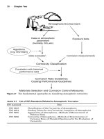
pipelines. The corrosion index was organized in three categories to
reflect three types of environment to which pipelines are exposed, i.e.,
atmospheric corrosion, soil corrosion, and internal corrosion. Table 4.3
contains the elements contributing to each type of environment and
the suggested weighting factors.
The basic risk assessment model can be expanded to incorporate
additional features that may be of concern in specific situations, as
illustrated in Fig. 4.13. Since these features do not necessarily apply
to all pipelines, this permits the use of distinct modules that can be
activated by an operator to modify the risk analysis.
4.2.3 Toward a universal model of materials
failure
One of the principal goals of scientific discovery is the development of a
theory, i.e., a coherent body of knowledge that can be used to provide

Modeling, Life Prediction, and Computer Applications 291
TABLE 4.3 Corrosion Risk Subjective Assessment
Problem Weight
Atmospheric corrosion
1. Facilities 0–5 pts
2. Atmospheric type 0–10 pts
3. Coating/inspection 0–5 pts
0–20 pts
Internal corrosion
1. Product corrosivity 0–10 pts
2. Internal protection 0–10 pts
0–20 pts
Soil corrosion
1. Cathodic protection 0–8 pts
2. Coating condition 0–10 pts
3. Soil corrosivity 0–4 pts
4. Age of system 0–3 pts
5. Other metals 0–4 pts
6. AC induced currents 0–4 pts
7. SCC and HIC 0–5 pts
8. Test leads 0–6 pts
9. Close internal surveys 0–8 pts
10. Inspection tool 0–8 pts
0–60 pts
Total 0–100 pts
0765162_Ch04_Roberge 9/1/99 4:43 Page 291
explanations and predictions for a specific domain of knowledge. Theory
development is a complex process involving three principal activities:
theory formation, theory revision, and paradigm shift. A theory is first
developed from a collection of known observations. It then goes through

a series of revisions aimed at reducing the shortcomings of the initial
model. The initial theory can thus evolve into one that can provide
sophisticated predictions. But a theory can also become much more com-
plex and difficult to use. In such cases, the problems can be partly elim-
inated by a paradigm shift, i.e., a revolutionary change that involves a
conceptual reorganization of the theory.
27
The Venn diagrams of Fig.
4.14 illustrate the three stages of a theory revision.
28
In the first stage
of theory revision, (a), an anomaly is noted, a new observation that is
not explained by the current model. In a subsequent stage, (b), the old
theory is reduced to its most basic or fundamental expression before it
finally serves as the basis of a new theory formulation, (c).
A sound corrosion failure model should thus be based on core prin-
ciples with extensions into real-world applications through adaptive
revision mechanisms. A universal representation describing the inter-
actions among defects, faults, and failures of a system is shown in Fig.
4.15. The arrows in this figure imply that quantifiable relations, char-
acteristic of a specific system, exist between a defect, a fault, and a
failure. The nature of various corrosion defects is introduced in Chap.
5, Corrosion Failures, in the section on forms of corrosion. Also in
Chap. 5, the factors causing these defects have been related to the fun-
292 Chapter Four
Cost of
service
interruption
module
Product hazard

Dispersion factor
Sabotage
module
Distribution
systems
Offshore
pipelines
Stress
module
Basic pipeline
risk assessment
model.
Third party
damage index
Leak
history
adjustment
Environmental
module
Failure mode
adjustment
Relative
Risk
Score
Corrosion
index
Design
index
Incorrect
operations

index
Index
Sum
Leak impact
factor
Data gathered
from records
and interviews
Figure 4.13 Optional modules to customize the basic pipeline risk assessment model.
0765162_Ch04_Roberge 9/1/99 4:43 Page 292