Handbook of Corrosion Engineering Episode 2 Part 13 doc

1035
TABLE D.4 Pure Species Considered and Their Thermodynamic Data
Species G
0
(298 K)
, Jиmol
Ϫ1
S
0
(298 K)
, Jиmol
Ϫ1
ABϫ 10
3
C ϫ 10
Ϫ5
C
p
,
*
Jиmol
Ϫ1
иK
Ϫ1
G
0
(333 K)
,† Jиmol
Ϫ1
O
2

0 205 29.96 4.184 1.674 29.85 Ϫ7,234.04
H
2
0 131 27.28 3.263 0.502 28.82 Ϫ4,642.01
H
2
O Ϫ237,000 69.9 10.669 42.284 Ϫ6.903 18.54 Ϫ239,483
Al 0 28.325 20.67 12.38 0 24.79 Ϫ1,040.43
Al(OH)
3
Ϫ1,136,542 0 Ϫ1,136,542
Al
2
O
3
иH
2
O Ϫ1,825,500 96.86 120.8 35.14 0 132.51 Ϫ1,829,152
*Calculated with Eq. (D.46).
†Calculated with Eq. (D.48).
0765162_AppD_Roberge 9/1/99 8:12 Page 1035
TABLE D.5 Soluble Species Considered and Their Thermodynamic Data
Species G
0
(298 K)
, S
0
(
298 K)
, S

ˇ 0
(298 K)
, ab C
p
,* G
0
(333 K)
,†
Jиmol
Ϫ1
Jиmol
Ϫ1
Jиmol
Ϫ1
Jиmol
Ϫ1
иK
Ϫ1
Jиmol
Ϫ1
H
ϩ
00Ϫ20.9 0.065 Ϫ0.005 118.75 Ϫ234.9
OH
Ϫ
Ϫ157,277 41.888 20.968 Ϫ0.37 0.0055 Ϫ452.03 Ϫ157,849
Al
3ϩ
Ϫ485,400 Ϫ321.75 Ϫ384.45 0.13 Ϫ0.00166 372.84 Ϫ474,876
Al(OH)

2ϩ
Ϫ694,100 Ϫ142.26 Ϫ184.06 0.13 Ϫ0.00166 267.95 Ϫ689,651
Al(OH)
2
ϩ
Ϫ900,000 205.35 184.43 0.13 Ϫ0.00166 75.06 Ϫ907,336
AlO
2
Ϫ
Ϫ838,968 96.399 117.31 Ϫ0.37 0.0055 Ϫ284.94 Ϫ841,778
*Calculated with Eq. (D.47).
†Calculated with Eq. (D.48).
1036
0765162_AppD_Roberge 9/1/99 8:12 Page 1036
G
0
(T
2
)
ϭ G
0
(T
1
)
Ϫ S
0
(T
1
)
[T

2
Ϫ T
1
] Ϫ T
2
͵
T
2
T
1
dT ϩ ͵
T
2
T
1
C
p
0
dT (D.45)
For pure substances (i.e., solids, liquids, and gases) the heat capaci-
ty C
p
0
is often expressed, as in Table D.4, as function of the absolute
temperature:
C
p
0
ϭ A ϩ BT ϩ CT
Ϫ2

(D.46)
For ionic substances, one has to use another method, such as pro-
posed by Criss and Cobble in 1964,
1
to obtain the heat capacity, provided
the temperature does not rise above 200°C. The expression of the ionic
capacity [Eq. (D.47)] makes use of absolute entropy values and the
parameters a and b contained in Table D.4:
C
p
0
ϭ (4.186a ϩ bS
0
(298 K)
) (T
2
Ϫ 298.16) /ln
΂΃
(D.47)
T
2
ᎏ
298.16
C
p
0
ᎏ
T
Electrochemistry Basics 1037
TABLE D.6 Reactions Considered to Model an Aluminum-Air Corrosion Cell

Water equilibria
2 e
Ϫ
ϩ 2 H
ϩ
ϭ H
2
4 e
Ϫ
ϩ O
2
ϩ 4 H
ϩ
ϭ 2 H
2
O
OH
Ϫ
ϩ H
ϩ
ϭ H
2
O
Equilibria involving aluminum metal
3 e
Ϫ
ϩ Al
3ϩ
ϭ Al
3 e

Ϫ
ϩ Al(OH)
3
ϩ 3 H
ϩ
ϭ Al ϩ 3 H
2
O
6 e
Ϫ
ϩ Al
2
O
3
иH
2
O ϩ 6 H
ϩ
ϭ 2 Al ϩ 4 H
2
O
3 e
Ϫ
ϩ AlO
2
Ϫ
ϩ 4 H
ϩ
ϭ Al ϩ 2 H
2

O
3 e
Ϫ
ϩ Al(OH)
2ϩ
ϩ H
ϩ
ϭ Al ϩ H
2
O
3 e
Ϫ
ϩ Al(OH)
2
ϩ
ϩ 2 H
ϩ
ϭ Al ϩ 2 H
2
O
Equilibria involving solid forms of oxidized aluminum
Al(OH)
3
ϩ H
ϩ
ϭ Al(OH)
2
ϩ
ϩ H
2

O
Al
2
O
3
иH
2
O ϩ 2 H
ϩ
ϭ 2 Al(OH)
2
ϩ
Al(OH)
3
ϩ 2 H
ϩ
ϭ Al(OH)
2ϩ
ϩ 2 H
2
O
Al
2
O
3
иH
2
O ϩ 4 H
ϩ
ϭ 2 Al(OH)

2ϩ
ϩ 2 H
2
O
Al(OH)
3
ϩ 3 H
ϩ
ϭ 2 Al
3ϩ
ϩ 4 H
2
O
Al
2
O
3
иH
2
O ϩ 6 H
ϩ
ϭ Al
3ϩ
ϩ 3 H
2
O
Al(OH)
3
ϭ AlO
2

Ϫ
ϩ H
ϩ
ϩ H
2
O
Al
2
O
3
иH
2
O ϭ 2 AlO
2
Ϫ
ϩ 2 H
ϩ
Equilibria involving only soluble forms of oxidized aluminum
AlO
2
Ϫ
ϩ 4 H
ϩ
ϭ Al
3ϩ
ϩ 2 H
2
O
0765162_AppD_Roberge 9/1/99 8:12 Page 1037
By combining Eq. (D.46) or (D.47) with Eq. (D.45) one can obtain the

free energy [Eq. (D.48)] at any given temperature by using the funda-
mental data contained in Tables D.4 and D.5:
G
0
(T)
ϭ G
0
(298 K)
ϩ (C
p
0
Ϫ S
0
(298 K)
) (T
2
Ϫ 298.16)
Ϫ T
2
ln
΂΃
C
p
0
(D.48)
Although these equations appear slightly overwhelming, they can be
computed relatively simply with the use of a modern spreadsheet,
where the data in Table D.4 could be imported with the functions in
Eqs. (D.46) to (D.48) properly expressed.
Calculate G for each species. For species O, the free energy of 1 mol can

be obtained from G
0
with Eq. (D.49):
G
o(T)
ϭ G
o(T)
0
ϩ 2.303 RT log
10
a
O
(D.49)
For x mol of species O the free energy is expressed by Eq. (D.50):
xG
0(T)
ϭ x (G
O(T)
0
ϩ 2.303 RT log
10
a
O
) (D.50)
For pure substances such as solids, a
O
is equal to 1. For a gas, a
O
is
equal to its partial pressure (p

O
), as a fraction of 1 atmosphere. For sol-
uble species, the activity of species O (a
O
), is the product of the activi-
ty coefficient of that species (␥
O
) with its molar concentration ([O]) (i.e.,
a
O
ϭ␥
O
[O]). The activity coefficient of a chemical species in solution is
close to 1 at infinite dilution when there is no interference from other
chemical species. For most other situations the activity coefficient is a
complex function that varies with the concentration of the species and
with the concentration of other species in solution. For the sake of sim-
plicity the activity coefficient will be assumed to be of value 1; hence
Eq. (D.50) can be written as a function of [O]:
xG
O(T)
ϭ x (G
O(T)
0
ϩ 2.303 RT log
10
[O]) (D.51)
Taking the global reaction fo the Al-O
2
system expressed in Eq.

(D.44) and the G
0
values calculated for 60°C in Tables D.4 and D.5, one
can obtain thermodynamic values for the products and reactants, as is
done in Table D.7.
Calculate cell ⌬G. The DG of a cell can be calculated by subtracting the
G values of the reactants from the G values of the products in Table
D.7. Keeping the example of the global reaction at 60°C in mind, one
would obtain
⌬G ϭ G
products
ϪG
reactants
ϭϪ3,846,087Ϫ (Ϫ670,615) ϭϪ3,175,472 J
T
2
ᎏ
298.16
1038 Appendix D
0765162_AppD_Roberge 9/1/99 8:12 Page 1038
Translate ⌬G into potential
E ϭϭ ϭ2.74 V
where n ϭ 12 because each Al gives off 3 e
Ϫ
[cf. Eq. (D.40)] and there
are four Al in the global Eq. (D.44) representing the cell chemistry.
Calculate the specific capacity (Ahиkg
Ϫ1
). The specific capacity relates the
weight of active materials with the charge that can be produced, that

is, a number of coulombs or ampere-hours (Ah). Because 1 A ϭ 1 Cиs
Ϫ1
,
1 Ah ϭ 3600 C, and because 1 mole of e
Ϫ
ϭ 96,485 C (Faraday), 1 mole
of e
Ϫ
ϭ 26.80 Ah.
By considering the global expression of the cell chemistry expressed
in Eq. (D.44), one can relate the weight of the active materials to a cer-
tain energy and power. In the present case 12 moles of e
Ϫ
are produced
by using
4 moles of Al 4 ϫ 26.98 gиmol
Ϫ1
, or 107.92 g
4 moles of OH
Ϫ
as KOH 4 ϫ 56.11 gиmol
Ϫ1
, or 224.44 g
3 moles of O
2
(as air) 0 g
3 moles of O
2
(compressed or cryogenic) 3 ϫ 32.00 g mol
Ϫ1

, or 96.00 g
Weight of active materials for the production of 12 moles of e
Ϫ
is then
332.36 g if running on free air and 428.36 g if running on compressed
or cryogenic oxygen. The theoretical specific capacity is thus 26.80 ϫ
12/0.3324 ϭ 967.5 Ahиkg
Ϫ1
if running on air and 26.80 ϫ 12/0.4284 ϭ
750.7 Ahиkg
Ϫ1
if running on compressed or cryogenic oxygen.
Calculate the energy density (Whиkg
Ϫ1
). The energy density can then be
obtained by multiplying the specific capacity obtained from calculating
the specific capacity with the thermodynamic voltage calculated when
3,188,818
ᎏᎏ
(12 и 96,485)
Ϫ⌬G
ᎏ
nF
Electrochemistry Basics 1039
TABLE D.7 Calculated Free Energies for Species Involved in the Global Al-Air
Reaction at 60°C
G
0
(333 K)
, 2.303RT

Species x Jиmol
Ϫ1
a
o
log
10
a
O
x G
0
(333 K)
∑G
0
(333 K)
Reactants
Al 4 Ϫ1040.43 1 0.00 Ϫ4161.72
OH
Ϫ
4 Ϫ157,849 1 0.00 Ϫ631,396.00
O
2
3 Ϫ7,234.04 0.2 Ϫ4452.02 Ϫ35,058.17 Ϫ670,615.89
Products
AlO
2
Ϫ
4 Ϫ841,778 0.1 Ϫ6369.39 Ϫ3,392,589.58
H
2
O2Ϫ239,483 1 0.00 Ϫ478,966.00 Ϫ3,846,087.21

0765162_AppD_Roberge 9/1/99 8:12 Page 1039
translating ⌬G into potentials: 2.74 ϫ 967.5 ϭ 2651 Whиkg
Ϫ1
, or 2.651
kWhиkg
Ϫ1
if running on air and, because the voltage for running on pure
oxygen is slightly higher (i.e., 2.78 V), 2.78 ϫ 750.7 ϭ 2087 Whиkg
Ϫ1
, or
2.087 kWhиkg
Ϫ1
if running on compressed or cryogenic oxygen.
Reference electrodes. The thermodynamic equilibrium of any other
chemical or electrochemical reaction can be calculated in the same man-
ner, provided the basic information is found. Table D.8 contains the
chemical description of most reference electrodes used in laboratories
and field units, and Tables D.9 and D.10, respectively, contain the ther-
modynamic data associated with the solid and soluble chemical species
making these electrodes. Table D.11 presents the results of the calcula-
tions performed to obtain the potential of each electrode at 60°C (i.e.,
away from the 25°C standard temperature).
D.2.6 Potential-pH diagrams
Potential-pH (E-pH) diagrams, also called predominance or Pourbaix
diagrams, have been adopted universally since their conception in the
early 1950s. They have been repetitively proven to be an elegant way
to represent the thermodynamic stability of chemical species in given
aqueous environments. E-pH diagrams are typically plotted for vari-
ous equilibria on normal cartesian coordinates with potential (E) as
the ordinate (y-axis) and pH as the abscissa (x-axis).

2
Pourbaix diagrams are a convenient way of summarizing much ther-
modynamic data, and they provide a useful means of predicting elec-
trochemical and chemical processes that could potentially occur in
certain conditions of pressure, temperature, and chemical makeup.
These diagrams have been particularly fruitful in contributing to the
understanding of corrosion reactions.
Stability of water. Equation (D.52) describes the equilibrium between
hydrogen ions and hydrogen gas in an aqueous environment:.
2H
ϩ
ϩ 2e
Ϫ
ϭ H
2
(D.52)
which can be written as Eq. (D.53) in neutral or alkaline solutions:
2H
2
O ϩ 2e
Ϫ
ϭ H
2
ϩ 2OH
Ϫ
(D.53)
Adding sufficient OH
Ϫ
to both sides of the reaction in Eq. (D.52)
results in Eq. (D.53). At higher pH than neutral, Eq. (D.53) is a more

appropriate representation. However, both representations signify the
same reaction for which the thermodynamic behavior can be expressed
by a Nernst Eq. (D.54):
1040 Appendix D
0765162_AppD_Roberge 9/1/99 8:12 Page 1040
TABLE D.8 Equilibrium Potential of the Main Reference Electrodes Used in Corrosion, at 25°C
Name Equilibrium reaction Nernst Equation, V vs. S H E Potential, V vs. S H E T coefficient, mVиC
Ϫ1
Hydrogen 2 H
ϩ
ϩ 2 e
Ϫ
ϭ H
2
(SHE) E
0
Ϫ 0.059 pH 0.00
Silver chloride AgCl ϩ e
Ϫ
ϭ Ag ϩ Cl
Ϫ
E
0
Ϫ 0.059 log
10
a
ClϪ
0.2224 Ϫ0.6
0.1 M KCl 0.2881
1.0 M KCl 0.2224

Seawater ϳ 0.250
Calomel Hg
2
Cl
2
ϩ 2 e
Ϫ
ϭ 2 Hg ϩ 2 Cl
Ϫ
E
0
Ϫ 0.059 log
10
a
Cl Ϫ
0.268
0.1 M KC1 0.3337 Ϫ0.06
1.0 M KC1 0.280 Ϫ0.24
(SCE) Saturated 0.241 Ϫ0.65
Mercurous sulfate Hg
2
SO
4
ϩ 2 e
Ϫ
ϭ 2 Hg ϩ SO
4
Ϫ2
E
0

Ϫ 0.0295 log
10
a
SO4
2 Ϫ
0.6151
Mercuric oxide Hg
O
ϩ 2 e
Ϫ
ϩ 2 H
ϩ
ϭ Hg ϩ H
2
OE
0
Ϫ 0.059 pH 0.926
Copper sulfate Cu
2ϩ
ϩ 2 e
Ϫ
ϭ Cu (sulfate solution) E
0
ϩ 0.0295 log
10
a
Cu
2ϩ
0.340
Saturated 0.318

1041
0765162_AppD_Roberge 9/1/99 8:12 Page 1041
TABLE D.9 Data and Calculations of t the Free Energy and Potential of the Main Reference Electodes at 60°C
(TemRef ϭ 25; TemC ϭ 60; TemA ϭ 333.16; T
2
Ϫ T
1
ϭ 35; ln(T
2
/T
1
) ϭ 0.1109926)
G
0
(298 K), S
0
(298 K), C
p
(333K),* G
0
T (333K),
†
Species Jиmol
Ϫ1
Jиmol
Ϫ1
AB CJиmol
Ϫ1
иK
Ϫ1

Jиmol
Ϫ1
O
2
0 205 29.96 4.184 Ϫ1.674 29.85 Ϫ7234.04
H
2
0 131 27.28 3.263 0.502 28.8 Ϫ4642.01
H
2
O Ϫ237000 69.9 10.669 42.284 Ϫ6.903 18.5 Ϫ239483.00
Ag 0 42.55 21.297 8.535 1.506 25.5 Ϫ1539.69
Cu 0 33.2 22.635 6.276 24.7 Ϫ1210.91
Hg 0 76.02 26.94 0 0.795 27.7 Ϫ2715.41
AgC1 Ϫ109805 96.2 62.258 4.184 Ϫ11.297 53.5 Ϫ113277.
Hg
2
C1
2
Ϫ210778 192.5 63.932 43.514 0 78.4 Ϫ217670.
Hg
2
SO
4
Ϫ625880 200.66 131.96 132 Ϫ633164.
HgO Ϫ58555 70.29 34.853 30.836 0 45.1 Ϫ61104.4
*Calculated with Eq. (D.46).
†Calculated with Eq. (D.48).
1042
0765162_AppD_Roberge 9/1/99 8:12 Page 1042

1043
TABLE D.10 Thermodynamic Data of Soluble Species Associated with the Most Commonly Used Reference
Electrodes
G
0
(298K), S
0
(298K), S
ˇ 0
(298K),
Species Jиmol
Ϫ1
Jиmol
Ϫ1
Jиmol
Ϫ1
abC
p
Eq.(D.47) Eq.(D.48)
H
ϩ
00Ϫ20.9 0.065 Ϫ0.005 118.7525 Ϫ234.927
Cu
2ϩ
65689 Ϫ207.2 Ϫ249.04 0.13 Ϫ0.00166 301.9618 72343.6
Cl
Ϫ
Ϫ131260 Ϫ12.6 8.32 Ϫ0.37 0.0055 Ϫ473.9694 Ϫ129881.
SO
4

2Ϫ
Ϫ744600 10.752 52.592 Ϫ0.37 0.0055 Ϫ397.1863 Ϫ744190.
0765162_AppD_Roberge 9/1/99 8:12 Page 1043
TABLE D.11 Calculations of the Equilibrium Associated with the Most Commonly Used Reference Electrodes at 60°C
ΑG° reactants,* ΑG° products,* ⌬G° reaction, Potential,
Name
J
и
mol
–1
J
и
mol
–1
J
и
mol
–1
V
Hydrogen –470 –46,420 –4,172 0.0216
Silver chloride –113,277 –131,421 –18,144 0.1880
Calomel –217,670 –265,193 –47,523 0.2463
Mercurous sulfate –633,164 –749,621 –116,457 0.6035
Mercuric chloride –61,574 –242,199 –180,624 0.9360
Copper sulfate 72,344 –1,211 –73,555 0.3812
*Note: all species considered to be of activity = 1
1044
0765162_AppD_Roberge 9/1/99 8:12 Page 1044
Electrochemistry Basics 1045
E

H
ϩ
/H
2
ϭ E
H
ϩ
/H
2
0
ϩ ln (D.54)
that becomes Eq. (D.55) at 25°C and p
H
2
of value unity:
E
H
ϩ
/H
2
ϭ E
H
ϩ
/H
2
0
Ϫ0.059 pH
(D.55)
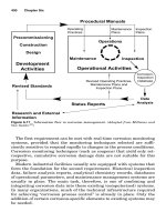
Equation (D.52) and its alkaline or basic form, Equation (D.53),
delineate the stability of water in a reducing environment and are

represented in a graphical form by the sloping line (a) on the
Pourbaix diagram in Fig. D.6. Below line (a) in this figure the equi-
librium reaction indicates that the decomposition of H
2
O into hydro-
gen is favored, whereas it is thermodynamically stable above that
line. As potential becomes more positive or noble, water can be
decomposed into its other constituent, oxygen, as illustrated in Eqs.
(D.56) and (D.57) for, respectively, the acidic form and neutral or
basic form of the same process:
O
2
ϩ 4H
ϩ
ϩ 4e
Ϫ
ϭ 2H
2
O (D.56)
O
2
ϩ 2H
2
O ϩ 4e
Ϫ
ϭ 4OH
Ϫ
(D.57)
Again these equivalent equations can be used to develop a Nernst
expression of the potential, that is Eq. (D.58) expressed as Eq. (D.59)

in standard conditions of temperature and oxygen pressure (i.e., p
O
2
of
value unity):
E
O
2
/H
2
O
ϭ E
O
2
/H
2
O
0
ϩ ln p
O
2
[H
ϩ
]
4
(D.58)
E
O
2
/H

2
O
ϭ E
O
2
/H
2
O
0
Ϫ 0.059 pH (D.59)
The line labeled (b) in Fig. D.6 represents the behavior of E vs. pH
for this last equation. Figure D.6 is divided into three regions. In the
upper one, water can be oxidized and form oxygen, whereas in the lower
one, it can be reduced to form hydrogen gas. In the intermediate
region, water is thermodynamically stable. It is common practice to
superimpose these two lines (a) and (b) on Pourbaix diagrams to mark
the water stability boundaries.
Predominance diagram of aluminum. Aluminum provides one of the
simplest cases for demonstrating the construction of E-pH diagrams.
In the following discussion, only four species containing the alu-
minum element will be considered: two solid species (Al and
Al
2
O
3
иH
2
O) and two ionic species (Al
3ϩ
and AlO

2
). The first equilibrium
RT
ᎏ
nF
[H
ϩ
]
2
ᎏ
p
H
2
RT
ᎏ
nF
0765162_AppD_Roberge 9/1/99 8:12 Page 1045
to consider examines the possible presence of either Al
3ϩ
or AlO
2
Ϫ
expressed in Eq. (D.60):.
Al
3 ϩ
ϩ 2H
2
O ϭ AlO
2
Ϫ

ϩ 4H
ϩ
(D.60)
Because there is no change in valence of the aluminum present in
the two ionic species considered, the associated equilibrium is inde-
pendent of the potential, and the expression of that equilibrium can
be derived to give an expression valid in standard conditions [Eq.
(D.61)]:
RT ln K
eq
ϭ RT ln Q ϭϪ⌬G
0
reaction
(D.61)
where
Q ϭ
a
AlO
2
Ϫ a
4
H
ϩ
ᎏᎏ
a
Al
3 ϩ
a
2
H

2
O
1046 Appendix D
-2
-20246810121416
-1.5
-1
-0.5
0
0.5
1
1.5
2
O
2
+ 4H
+
+ 4e
-
= 2H
2
O
b
a
Potential (V vs. SHE)
2H
+
+ 2e
-
= H

2
O
2
OH
-
+ H
+
= H
2
O
H
2
pH
Figure D.6 Stability diagram of water at 25°C.
0765162_AppD_Roberge 9/1/99 8:12 Page 1046
Assuming that the activity of H
2
O is unity and that the activities of
the two ionic species are equal, one can obtain a simpler expression of
the equilibrium based purely on the activity of H
ϩ
:
4 log
10
[H
ϩ
] ϭ (D.62)
or, if G
0
is expressed in joules,

Ϫ4 log
10
[H
ϩ
] ϭ 4 pH ϭ⌬G
0
reaction
ϫ 1.75 ϫ 10
Ϫ4
(D.63)
By using the thermodynamic data provided in Tables D.4 and D.5
and following the detailed procedure outlined earlier, it is possible to
calculate that the free energy of reaction [Eq. (D.60)] is in fact equal to
120.44 kJиmol
Ϫ1
(for either 1 [Al
3ϩ
] or 1 [AlO
2
Ϫ
]). Equation (D.63) then
becomes Equation (D.64):
pH ϭ 120,440 ϫ 4.38 ϫ 10
Ϫ5
ϭ 5.27 (D.64)
This is represented, in the E-pH diagram shown in Fig. D.7, by a
dotted vertical line separating the dominant presence of Al
3ϩ
at low pH
from the dominant presence of AlO

2
Ϫ
at the higher end of the pH scale.
The next phase for constructing the aluminum E-pH diagram is to
consider the equilibria between the four species mentioned earlier. A
computer program that would compare all possible interactions and
rank them in terms of their thermodynamic stability would typically
carry out this work. The steps of this data-crunching process are illus-
trated in Figs. D.8 to D.10.
D.3 Kinetic Principles
Thermodynamic principles can help explain a situation in terms of the
stability of chemical species and reactions associated with corrosion
process. However, thermodynamic calculations cannot be used to pre-
dict reaction rates. Electrode kinetic principles have to be used to esti-
mate these rates.
D.3.1 Kinetics at equilibrium: The
exchange current concept
The exchange current I
o
is a fundamental characteristic of electrode
behavior that can be defined as the rate of oxidation or reduction at an
equilibrium electrode expressed in terms of current. Exchange cur-
rent, in fact, is a misnomer because there is no net current flow. It is
merely a convenient way of representing the rates of oxidation and
Ϫ⌬G’
0
reaction
ᎏᎏ
2.303RT
Electrochemistry Basics 1047

0765162_AppD_Roberge 9/1/99 8:12 Page 1047
reduction of a given electrode at equilibrium, when no loss or gain is
experienced by the electrode material. As an example, the exchange
current for reducing ferric ions, Eq. (D.65), would be related to the cur-
rent of each direction of a reversible reaction, that is, a cathodic
branch (I
c
) representing Eq. (D.65) and an anodic current (I
a
) repre-
senting Eq. (D.66):
Fe
3 ϩ
ϩ 1e
Ϫ
→ Fe
2 ϩ
(D.65)
Fe
2 ϩ
→ Fe
3 ϩ
ϩ 1e
Ϫ
(D.66)
Because the net current is zero at equilibrium, it implies that the
sum of these two currents is zero as in Eq. (D.67). Because I
a
is, by con-
vention, always positive, it follows that, when no external voltage or

current is applied to the system, the exchange current I
o
is equal to I
c
or I
a
[Eq. (D.68)]:
1048 Appendix D
-2
-2 0 2 4 6 8 10 12 14 16
-1.5
-1
-0.5
0
0.5
1
1.5
2
b
a
Potential (V vs. SHE)
AlO
2
-
Al
3+
pH
Al
3+
+ 2H

2
O = AlΟ
2
-
+ 4H
+
Figure D.7 Equilibrium diagram of Al-soluble species.
0765162_AppD_Roberge 9/1/99 8:12 Page 1048
I
a
ϩ I
c
ϭ 0 (D.67)
I
a
ϭϪI
c
ϭ I
o
(D.68)
There is no theoretical way of accurately determining the exchange
current for any given system. This must be determined experimentally.
For the characterization of electrochemical processes it is always
preferable to normalize the value of the current by the surface area of
the electrode and use the current density often expressed as a small i
(i.e., i ϭ I/surface area).
D.3.2 Kinetics under polarization
Electrodes can be polarized by the application of an external voltage or
by the spontaneous production of a voltage away from equilibrium.
This deviation from equilibrium potential is called polarization. The

Electrochemistry Basics 1049
-2
-2 0 2 4 6 8 10 12 14 16
-1.5
-1
-0.5
0
0.5
1
1.5
2
b
a
Potential (V vs. SHE)
pH
Al
2
O
3
.H
2
O
Al
[Al
3+
] = 1 M
[AlO
2
-
] = 1 M

Figure D.8 Equilibrium diagram of Al solid species when soluble species are at a 1-molar
concentration.
0765162_AppD_Roberge 9/1/99 8:12 Page 1049
magnitude of polarization is usually described as an overvoltage (␩),
that is, a measure of polarization with respect to the equilibrium
potential (E
eq
) of an electrode. This polarization is said to be either
anodic, when the anodic processes on the electrode are accelerated by
changing the specimen potential in the positive (noble) direction, or
cathodic, when the cathodic processes are accelerated by moving the
potential in the negative (active) direction. There are three distinct
types of polarization in any electrochemical cell, the total polarization
across an electrochemical cell being the summation of the individual
elements as expressed in Eq. (D.69):
E
applied
Ϫ E
eq
ϭ␩
total
ϭ␩
act
ϩ␩
conc
ϩ iR (D.69)
where ␩
act
ϭ activation overpotential, a complex function describing
the charge transfer kinetics of the electrochemical

1050 Appendix D
-2
-2 0 2 4 6 8 10 12 14 16
-1.5
-1
-0.5
0
0.5
1
1.5
2
b
a
Potential (V vs. SHE)
pH
Al
2
O
3
.H
2
O
Al
[Al
3+
] = 10
-2
M
[AlO
2

-
] = 10
-2
Figure D.9 Equilibrium diagram of Al solid species when soluble species are at a 10
Ϫ2
-
molar concentration.
0765162_AppD_Roberge 9/1/99 8:12 Page 1050
processes. ␩
act
is predominant at small polarization cur-
rents or voltages.
␩
conc
ϭ concentration overpotential, a function describing the
mass transport limitations associated with electrochem-
ical processes. ␩
conc
is predominant at large polarization
currents or voltages.
iR ϭ is often called the ohmic drop. iR follows Ohm’s law and
describes the polarization that occurs when a current
passes through an electrolyte or through any other
interface such as surface film, connectors, and so forth.
Activation polarization. Both the anodic and cathodic sides of a reac-
tion can be studied individually by using some well-established elec-
trochemical methods where the response of a system to an applied
polarization, current or voltage, is studied. A general representation of
Electrochemistry Basics 1051
-2

-2 0 2 4 6 8 10 12 14 16
-1.5
-1
-0.5
0
0.5
1
1.5
2
b
a
Potential (V vs. SHE)
pH
Al
2
O
3
.H
2
O
Al
Al
3+
AlO
2
-
10
-2
10
0

10
-6
10
-4
10
-2
10
0
10
-4
10
-6
Figure D.10 Equilibrium diagram of Al solid species when soluble species are at a 10
Ϫ6
molar concentration.
0765162_AppD_Roberge 9/1/99 8:12 Page 1051
the polarization of an electrode supporting one redox system is given
in the Butler-Volmer equation:.
i ϭ i
0
Ά
exp
΂
␤␩
act
΃
Ϫexp
΂
Ϫ (1Ϫ␤) ␩
act

΃·
(D.70)
where: i ϭ anodic or cathodic current.
␤ϭcharge transfer barrier or symmetry coefficient for the
anodic or cathodic reaction. ␤ values are typically close to
0.5.
␩
act
ϭ E
applied
Ϫ E
eq
(i.e., positive for anodic polarization and
negative for cathodic polarization).
n ϭ number of participating electrons.
R ϭ gas constant.
T ϭ absolute temperature.
F ϭ Faraday.
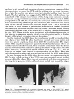
A polarization plot of the ferric/ferrous oxydo-reduction reaction on
palladium (i
o
10
0.8
mAиcm
Ϫ2
), iridium (i
o
10
0.2
mAиcm

Ϫ2
), and rhodium
(i
o
10
Ϫ4.8
mAиcm
Ϫ2
) is shown in Fig. D.11. The current behavior in Fig.
D.11 illustrates the high level of sensitivity of an electrode polarization
behavior to even small variations in the exchange current density. The
exchange current density reflects the electrocatalytic performance of
that electrode toward a specific reaction and can vary over many
orders of magnitude. The current density scale in Fig. D.11 had to be
changed to much lower values in Fig. D.12 to be able to see the current
behavior of the same reaction on rhodium.
The exchange current density for the production of hydrogen on a
metallic surface can similarly vary between 10
Ϫ2
Aиcm
Ϫ2
, for a good
electrocatalytic surface such as platinum, to as low as 10
Ϫ13
Aиcm
Ϫ2
for
electrode surfaces containing lead or mercury. Added, even in small
quantities, to battery electrode materials, mercury will stifle the dan-
gerous production of confined gaseous hydrogen. Mercury and lead

were also, for the same hydrogen-inhibiting property, commonly used
in many commercial processes as electrode material before their high
toxicity was acknowledged a few years ago. It should be noted that the
voltage on the polarization plots in Figs. D.11 and D.12 was presented
as the overvoltage, with current reversal of its polarity at zero. Figure
D.13 shows the data presented in Fig. D.11 with the absolute potential
instead of the overvoltage.
The presence of two polarization branches in a single reaction is
illustrated in Fig. D.14 for the same Fe
ϩ3
/Fe
ϩ2
couple in contact
with a palladium electrode. When ␩
act
is anodic (i.e., positive), the
second term in the Butler-Volmer equation becomes negligible, and
nF
ᎏ
RT
nF
ᎏ
RT
1052 Appendix D
0765162_AppD_Roberge 9/1/99 8:12 Page 1052
i
a
can be more simply expressed by Eq. (D.71) and its logarithm
form [Eq. (D.72)]:
i

a
ϭ i
o
Ά
exp
΂
␤
a
␩
a
΃·
(D.71)
␩
a
ϭ b
a
log
10
΂΃
(D.72)
where b
a
is the Tafel coefficient that can be obtained from the slope
[Eq. (D.73)] of a plot of ␩ against log i, with the intercept yielding a val-
ue for i
o
:
b
a
ϭ 2.303 и (D.73)

Similarly, when ␩
reaction
is cathodic (i.e., negative), the first term in
the Butler-Volmer equation becomes negligible, and i
c
can be more
RT
ᎏ
␤nF
i
a
ᎏ
i
o
nF
ᎏ
RT
Electrochemistry Basics 1053
-30
-25
-20
-15
-10
-5
0
5
10
15
20
25

30
-0.5-0.4-0.3-0.2-0.100.10.20.30.40.5
Current density (mA cm
-2
)
Overpotential (V)
i
o
= 10
0.8
i
o
= 10
0.2
i
o
= 10
-4.8
Figure D.11 Current vs. overvoltage polarization plot of the ferric/ferrous ion reaction on palladi-
um (i
o
ϭ 10
0.8
mAиcm
Ϫ2
), iridium (i
o
ϭ 10
0.2
mAиcm

Ϫ2
), and rhodium (i
o
ϭ 10
Ϫ4.8
mAиcm
Ϫ2
) on a
current scale of 60 mA.
0765162_AppD_Roberge 9/1/99 8:12 Page 1053
simply expressed by Eq. (D.74) and its logarithm [Eq. (D.75)], with b
c
obtained by plotting ␩ vs. log i [Eq. (D.76)]:
i
c
ϭ i
o
Ά
Ϫexp
΂
Ϫ (1Ϫ␤
c
) ␩
c
΃·
(D.74)
␩
c
ϭ b
c

log
10
΂΃
(D.75)
b
c
ϭϪ2.303 (D.76)
A Tafel plot for the same data set that was presented in Fig. D.14
is now shown in Fig. D.15 as a log (i)/overpotential plot. It is rela-
tively simple, using such representation, to obtain the exchange cur-
rent density values and the parameters behind the slopes of the
current/voltage behavior, that is, Eq. (D.76).
RT
ᎏ
␤nF
i
c
ᎏ
i
o
nF
ᎏ
RT
1054 Appendix D
-0.0003
-0.0002
-0.0001
0
0.0001
0.0002

0.0003
-0.5-0.4-0.3-0.2-0.100.10.20.30.40.5
Current density (mA cm
-2
)
Overpotential (V)
i
o
= 10
0.8
i
o
= 10
0.2
i
o
= 10
-4.8
Figure D.12 Current vs. overvoltage polarization plot of the ferric/ferrous ion reaction on palladi-
um (i
o
ϭ 10
0.8
mAиcm
Ϫ2
), iridium (i
o
ϭ 10
0.2
mAиcm

Ϫ2
), and rhodium (i
o
ϭ 10
Ϫ4.8
иmA cm
Ϫ2
) on a
current scale of 0.6 mA.
0765162_AppD_Roberge 9/1/99 8:12 Page 1054
Concentration polarization. When the cathodic reagent at the corroding
surface is in short supply, the mass transport of this reagent could
become rate controlling. A frequent case of this type of control occurs
when the cathodic processes depend on the reduction of dissolved oxygen.
Because the rate of the cathodic reaction is proportional to the surface
concentration of the reagent, the reaction rate will be limited by a drop
in the surface concentration. For a sufficiently fast charge transfer
(small activation overvoltage), the surface concentration will fall to zero,
and the corrosion process will be totally controlled by mass transport.
For purely diffusion-controlled mass transport, the flux of a species O to
a surface from the bulk is described with Fick’s first law [Eq. (D.77)]:
J
O
ϭϪD
O
΂΃
(D.77)
where J
O
ϭ flux of species O (mol s

Ϫ1
и cm
Ϫ2
)
D
O
ϭ diffusion coefficient of species O (cm
2
и s
Ϫ1
)
␦C
O
/␦x ϭ concentration gradient of species O across the inter-
face (mol и cm
Ϫ4
)
␦C
O
ᎏ
␦x
Electrochemistry Basics 1055
-30
-25
-20
-15
-10
-5
0
5

10
15
20
25
30
0.270.370.470.570.670.770.870.971.071.171.27
Current density (mA cm
-2
)
Potential (V vs. SHE)
i
o
= 10
0.8
i
o
= 10
0.2
i
o
= 10
-4.8
Figure D.13 Current vs. potential polarization plot of the ferric/ferrous ion reaction on palladium
(i
o
ϭ 10
0.8
mAиcm
Ϫ2
), iridium (i

o
ϭ 10
0.2
mAиcm
Ϫ2
), and rhodium (i
o
ϭ 10
Ϫ4.8
mAиcm
Ϫ2
) current
scale of 60 mA.
0765162_AppD_Roberge 9/1/99 8:12 Page 1055
The diffusion coefficient of an ionic species at infinite dilution can be
estimated with the help of Nernst-Einstein Eq. (D.78), relating D
O
with the conductivity of the species (␭
O
):
D
O
ϭ (D.78)
where z
O
ϭ the valency of species O
R ϭ gas constant (i.e., 8.314 J mol
Ϫ1
и K
Ϫ1

)
T ϭabsolute temperature (K)
F ϭ Faraday’s constant (i.e., 96487 C и mol
Ϫ1
)
Table 1.6 (Aqueous Corrosion) contains values for D
O
and ␭
O
of some
common ions. For more practical situations the diffusion coefficient
can be approximated with the help of Eq. (D.79), which relates D
O
to
the viscosity of the solution (␮) and absolute temperature:
D
O
ϭ (D.79)
where A is a constant for the system.
TA
ᎏ
␮
RT ␭
O
ᎏ
|z
O
|
2
F

2
1056 Appendix D
anodic branch
cathodic
-0.5-0.4-0.3-0.2-0.100.10.20.30.40.5
Current density (mA cm
-2
)
Overpotential (V)
i
o
= 10
0.8
mA cm
-2
-30
-25
-20
-15
-10
-5
0
5
10
15
20
25
30
Figure D.14 Current vs. overvoltage polarization plot of the ferric/ferrous ion reaction on pal-
ladium showing both the anodic and cathodic branches of the resultant current behavior.

0765162_AppD_Roberge 9/1/99 8:12 Page 1056
The region near the metallic surface where the concentration gradient
occurs is also called the diffusion layer (␦). Because the concentration
gradient ␦C
O
/␦x is greatest when the surface concentration of species O
is completely depleted at the surface (i.e., C
O
ϭ 0), it follows that the
cathodic current is limited in that condition, as expressed by Eq. (D.80):
i
c
ϭ i
L
ϭϪnFD
O
(D.80)
For intermediate cases, ␩
conc
can be evaluated using an expression
[Eq. (D.81)] derived from the Nernst equation:
␩
conc
ϭ log
10
(1 Ϫ ) (D.81)
where 2.303RT/F ϭ 0.059 V when T ϭ 298.16 K.
When concentration control is added to a process, it simply adds to
the polarization as in the following equation:
i

ᎏ
i
L
2.303RT
ᎏᎏ
nF
C
O
bulk
ᎏ
␦
Electrochemistry Basics 1057
0
0.5
1
1.5
2
2.5
3
-1-0.8-0.6-0.4-0.200.20.40.60.81
Anodic branch
Anodic slope
Cathodic slope
Cathodic branch
Log (Current density (mA cm
-2
))
Overpotential (V)
Log (i
o

)
Figure D.15 Log (current) vs. overvoltage Tafel plot of the ferric/ferrous ion reaction on palladi-
um showing how to obtain the exchange current density (intercept) and the slope b ϭϪ2.303
(RT/ßnF) of both the anodic and cathodic branches.
0765162_AppD_Roberge 9/1/99 8:12 Page 1057
␩
tot
ϭ␩
act
ϩ␩
conc
We know that, for purely activation controlled systems, the current
can be derived from the voltage with the following expression:
I ϭ 10
[ (E Ϫ E
eq
)
/
b
ϩ log
10
(I
o
) ]
To simplify the expression of the current in the presence of concentra-
tion effects, suppose that
A ϭ 10
[ (E Ϫ E
eq
)

/
b
ϩ log
10
(I
o
) ]
␩
tot
ϭ E Ϫ E
eq
ϭ␩
act
ϩ␩
conc
and
I ϭ
where I
l
is the limiting current of the cathodic process.
I
l
A
ᎏ
I
l
ϩ A
1058 Appendix D
-100
-80

-60
-40
-20
0
20
40
60
80
100
-1.5-1.3-1.1-0.9-0.7-0.5-0.3-0.10.10.30.50.70.91.11.31.5
Current density (mA cm
-2
)
Overpotential (V)
i
o
= 10
0.8
mA cm
-2
i
l
= 5 mA cm
-2
i
l
= 100 mA cm
-2
i
l

= 20 mA cm
-2
Figure D.16 Current vs. overvoltage epolarization plot of the ferric/ferrous ion reaction on palladi-
um with three levels of concentration overvoltage (100, 20, and 5 mAиcm
Ϫ2
).
0765162_AppD_Roberge 9/1/99 8:12 Page 1058
Figure D.6 illustrates the effect of a limiting current on the polar-
ization of an electrode. For this example three arbitrary limiting cur-
rent densities were added the activation voltage of the Fe
3ϩ
/Fe
2ϩ
reaction on palladium. Figure D.7 presents the same data set on a log-
arithmic current scale.
Ohmic overpotential. The ohmic drop caused by the electrolytic resis-
tance between two electrodes can be measured by using an alternating
current technique (see Sec. D.1.2, Electrolyte Conductance) or minimized
by measuring the potential as close as possible to the working electrode.
In any case the ohmic overpotential is a simple function described by the
product of the effective solution resistance and the cell current, or iR.
References
1. Criss, C. M., and Cobble, J. W., The Thermodynamic Properties of High Temperature
Aqueous Solutions, Journal of the American Chemical Society, 86:5385–5393 (1964).
2. Pourbaix, M., Atlas of Electrochemical Equilibria in Aqueous Solutions, Houston,
Tex., NACE International, 1974.
Electrochemistry Basics 1059

0
0.2

0.4
0.6
0.8
1
1.2
1.4
1.6
1.8
2
2.2
2.4
-1.5-1.3-1.1-0.9-0.7-0.5-0.3-0.10.10.30.50.70.91.11.31.5
Log (current density (mA cm
-2
))
Overpotential (V)
i
o
= 10
0.8
mA cm
-2
i
l
= 5 mA cm
-2
i
l
= 100 mA cm
-2

i
l
= 20 mA cm
-2
Figure D.17 Log (current) vs. overvoltage polarization plot of the ferric/ferrous ion reaction on pal-
ladium with three levels of concentration overvoltage (100, 20, and 5 mAиcm
Ϫ2
).
0765162_AppD_Roberge 9/1/99 8:12 Page 1059