C++ Programming for Games Module II phần 2 pot
Bạn đang xem bản rút gọn của tài liệu. Xem và tải ngay bản đầy đủ của tài liệu tại đây (1017.23 KB, 47 trang )
24
Introduction
Throughout most of the previous chapters, we have assumed that all of our code was designed and
implemented correctly and that the results could be anticipated. For example, we assumed that the user
entered the expected kind of input, such as a string when a string was expected or a number when a
number was expected. Additionally, we assumed that the arguments we passed into function parameters
were valid. But this may not always be true. For example, what happens if we pass in a negative integer
into a factorial function, which expects an integer greater than or equal to zero? Whenever we allocated
memory, we assumed that the memory allocation succeeded, but this is not always true, because
memory is finite and can run out. While we copied strings with strcpy, we assumed the destination
string receiving the copy had enough characters to store a copy, but what would happen if it did not?
It would be desirable if everything worked according to plan; however, in reality things tend to obey
Murphy’s Law (which paraphrased says “if anything can go wrong, it will”). In this chapter, we spend
some time getting familiar with several ways in which we can catch and handle errors. The overall goal
is to write code that is easy to debug, can (possibly) recover from errors, and exits gracefully with useful
error information if the program encounters a fatal error.
Chapter Objectives
• Understand the method of catching errors via function return codes, and an understanding of the
shortcomings of this method.
• Become familiar with the concepts of exception handling, its syntax, and its benefits.
• Learn how to write assumption verification code using asserts.
11.1 Error Codes
The method of using error codes is simple. For every function or method we write, we have it return a
value which signifies whether the function/method executed successfully or not. If it succeeded then we
return a code that signifies success. If it failed then we return a predefined value that specifies where
and why the function/method failed.
Let us take a moment to look at a real world example of an error return code system. In particular, we
will look at the system used by DirectX (a code library for adding graphics, sound, and input to your
applications). Consider the following DirectX function:
HRESULT WINAPI D3DXCreateTextureFromFile(
LPDIRECT3DDEVICE9 pDevice,
LPCTSTR pSrcFile,
LPDIRECT3DTEXTURE9 *ppTexture
);
25
Do not worry about what this function does or the data types this function uses, which you are not
familiar with.
This function has a return type HRESULT, which is simply a numeric code that identifies the success of
the function or an error. For instance, D3DXCreateTextureFromFile can return one of the following
return codes, which are defined numerically (i.e., the symbolic name represents a number). Which one
it returns depends upon what happens inside the function.
• D3D_OK: This return code means that the function executed completely successfully.
• D3DERR_NOTAVAILABLE: This return code means that the hardware cannot create a texture; that
is, texture creation is an “unavailable” feature. This is a failure code.
•
D3DERR_OUTOFVIDEOMEMORY: This return code means that there is not enough video memory
to put the texture in. This is a failure code.
•
D3DERR_INVALIDCALL: This return code means that the arguments passed into the parameters
are invalid. For example, you may have passed in a null pointer when the function expects a
valid pointer. This is a failure code.
• D3DXERR_INVALIDDATA: This return code means the source data (that is, the texture file) is not
valid. This error could occur if the file is corrupt, or we specified a file that is not actually a
texture file. This is a failure code.
• E_OUTOFMEMORY: This return code means there was not enough available memory to perform
the operation. This is a failure code.
By examining the return codes from functions that return error codes, we can figure out if an error
occurred, what potentially caused the error, and then respond appropriately. For example, we can write
the following code:
HRESULT hr = D3DXCreateTextureFromFile([ ]);
// Did an error occur?
if( hr != D3D_OK )
{
// Yes, find our which specific error
if( hr == D3DERR_NOTAVAILABLE )
{
DisplayErrorMsg("D3DERR_NOTAVAILABLE");
ExitProgram();
}
else if( hr == D3DERR_OUTOFVIDEOMEMORY )
{
DisplayErrorMsg("D3DERR_OUTOFVIDEOMEMORY");
ExitProgram();
}
else if( hr == D3DERR_INVALIDCALL )
{
26
DisplayErrorMsg("D3DERR_INVALIDCALL");
ExitProgram();
}
else if( hr == D3DXERR_INVALIDDATA )
{
DisplayErrorMsg("D3DXERR_INVALIDDATA");
ExitProgram();
}
else if( hr == E_OUTOFMEMORY )
{
DisplayErrorMsg("E_OUTOFMEMORY");
ExitProgram();
}
}
Here we simply display the error code to the user and then exit the program. Note that
DisplayErrorMsg and ExitProgram are functions you would have to implement yourself. They are
not part of the standard library.
11.2 Exception Handling Basics
One of the shortcomings of error codes is that for a single function call, we end up writing a lot of error
handling code, thereby bloating the size of the program. For example, at the end of the previous section
we saw that there were many lines of error handling code for a single function call. The problem
becomes worse on a larger scale:
FunctionCallA();
// Handle possible error codes
FunctionCallB();
// Handle possible error codes
FunctionCallC();
// Handle possible error codes
Such a style of mixing error-handling code in with non-error-handling code becomes so cumbersome
that it is seldom religiously followed throughout a program, and therefore, the program becomes unsafe.
C++ provides an alternative error-handling solution called exception handling.
Exception handling works like this: in a segment of code, if an error or something unexpected occurs,
the code throws an exception. An exception is represented with a class object, and as such, can do
anything a normal C++ class object can do. Once an exception has been thrown, the call stack unwinds
(a bit like returning from functions) until it finds a catch block that handles the exception. Let us look at
an example:
27
Program 11.1: Exception Handling.
#include <iostream>
#include <string>
using namespace std;
class DivideByZero
{
public:
DivideByZero(const string& s);
void errorMsg();
private:
string mErrorMsg;
};
DivideByZero::DivideByZero(const string& s)
{
mErrorMsg = s;
}
void DivideByZero::errorMsg()
{
cout << mErrorMsg << endl;
}
float Divide(float numerator, float denominator)
{
if( denominator == 0.0f )
throw DivideByZero("Divide by zero: result undefined");
return numerator / denominator;
}
int main()
{
try
{
float quotient = Divide(12.0f, 0.0f);
cout << "12 / 0 = " << quotient << endl;
}
catch(DivideByZero& e)
{
e.errorMsg();
}
}
Program 11.1 Output
Divide by zero: result undefined
Press any key to continue
The very first thing we do is define an exception class called DivideByZero. Remember that an
exception class is just like an ordinary class, except that we use instances of it to represent exceptions.
28
The next item of importance is in the Divide function. This function tests for a “divide by zero” and if
it occurs, we then construct and throw a DivideByZero object exception. Finally, in the main
function, in order to catch an exception we must use a try-catch block. In particular, we wrap the code
that can potentially throw an exception in the
try block, and we write the exception handling code in
the catch block. Note that the catch block takes an object. This object is the exception we are
looking to catch and handle.
It is definitely possible, and quite common, that a function or method will throw more than one kind of
exception. We can list catch statements so that we can handle the different kinds of exceptions:
try
{
SomeFunction();
}
catch(LogicError& logic)
{
// Handle logic error exception
}
catch(OutOfMemory& outOfMem)
{
// Handle out of memory exception
}
catch(InvalidData& invalid)
{
// Handle invalid data
}
In addition to a chain of catches, we can “catch any exception” by specifying an ellipses argument:
try{
SomeFunction();
}
catch( ){
// Generic error handling code
}
We can state two immediate benefits of exception handling.
1. The error-handling code (i.e., the catch block) is not intertwined with non-error-handling code; in
other words, we move all error handling code into a catch block. This is convenient from an
organizational standpoint.
2. We need not handle a thrown exception immediately; rather the stack will unwind until it finds a
catch block that handles the exception. This is convenient because, as functions can call other
functions, which call other functions, and so on, we do not want to have error handling code after
every function/method. Instead, with exceptions we can catch the exception at, say, the top level
function call, and any exception thrown in the inner function calls will eventually percolate up to
the top function call which can catch the error.
As a final note, be aware that this section merely touched on the basics of exception handling, and there
are many more details and special situations that can exist. Also note that the functionality of exception
handling is not free, and introduces some (typically minor) performance overhead.
29
11.3 Assert
In general, your functions and methods make certain assumptions. For example, a “print array” function
might assume that the program passes a valid array argument. However, it is possible that you might
have forgotten to initialize an array, and consequently, passed in a null pointer to the “print array”
function, thus causing an error. We could handle this problem with a traditional error handling system
as described in the previous two sections. However, such errors should not be occurring as the program
reaches completion. That is, if you are shipping a product that has a null pointer because you forgot to
initialize it then you should not be shipping the product to begin with. Error handling should be for
handling errors that are generally beyond the control of the program, such as missing or corrupt data
resources, incompatible hardware, unavailable memory, flawed input data, and so on.
Still, for debugging purposes, it is very convenient to have self-checks littered throughout the program
to ensure certain assumptions are true, such as the validity of a pointer. However, based on the previous
argument, we should not need these self-checks once we have agreed that the software is complete. In
other words, we want to remove these checks in the final version of the program. This is where assert
comes in.
To use the assert function you must include the standard library <cassert>. The assert function
takes a single boolean expression as an argument. If the expression is true then the assertion passes;
what was asserted is true. Conversely, if the expression evaluates to false then the assertion fails and a
dialog box like the one depicted in Figure 11.1 shows up, along with an assertion message in the console
window:
Figure 11.1: Assert message and dialog.
30
The information the assertion prints to the console is quite useful for debugging; it displays the condition
that failed, and it displays the source code file and line number of the condition that failed.
The key fact about asserts is that they are only used in the debug version of a program. When you
switch the compiler into “release mode” the assert functions are filtered out. This satisfies what we
previously sought when we said: “[…] we want to remove these checks [asserts] in the final version
of the program.”
To conclude, let us look at a complete, albeit simple, program that uses asserts.
Program 11.2: Using assert.
#include <iostream>
#include <cassert>
#include <string>
using namespace std;
void PrintIntArray(int array[], int size)
{
assert( array != 0 ); // Check for null array.
assert( size >= 1 ); // Check for a size >= 0.
for(int i = 0; i < size; ++i)
cout << array[i] << " ";
cout << endl;
}
int main()
{
int* array = 0;
PrintIntArray(array, 10);
}
The function
PrintIntArray makes two assumptions:
1) The array argument points to something (i.e., it is not null)
2) The array has a size of at least one element.
Both of these assumptions are asserted in code:
// Check for null array.
assert( array != 0 );
// Check for a size >= 0.
assert( size >= 1 );
Because we pass a null pointer into
PrintIntArray, in main, the assert fails and the dialog box and
assert message as shown in Figure 11.1 appear. As an exercise, correct the problem and verify that the
assertion succeeds.
31
11.4 Summary
1. When using error codes to handle errors for every function or method we write, we have it return
a value, which signifies whether the function/method executed successfully or not. If it
succeeded then we return a code that signifies success. If it failed then we return a predefined
value that specifies where and why the function/method failed. One of the shortcomings of error
codes is that for a single function call, we end up writing much more error handling code,
thereby bloating the size of the program.
2. Exception handling works like this: in a segment of code, if an error or something unexpected
occurs, the code throws an exception. An exception is represented with a class object, and as
such, can do anything a normal C++ class object can do. Once an exception has been thrown,
the stack unwinds (a bit like returning from functions) until it finds a catch block that handles the
exception. One of the benefits of exception handling is that the error-handling code (i.e., the
catch block) is not intertwined with non-error-handling code; in other words, we move all error
handling code into a catch block. This is convenient from an organizational standpoint. Another
benefit of exception handling is that we need not handle a thrown exception immediately; rather
the stack will unwind until it finds a catch block that handles the exception. This is convenient
because, as functions can call other functions, which call other functions, and so on, we do not
want to have error handling code after every function/method. Instead, with exceptions we can
catch the exception at the top level function call, and any exception thrown in the inner function
calls will eventually percolate up to the top function call which can catch the error. Be aware
that the functionality of exception handling is not free, and introduces some performance
overhead.
3. To use the assert function, you must include the standard library <cassert>. The assert
function takes a single boolean expression as an argument. If the expression is true then the
assertion passes; what was asserted is true. Conversely, if the expression evaluates to false then
the assertion fails and a message is displayed along with a dialog box. The key fact about
asserts is that they are only used in the debug version of a program. When you switch the
compiler into “release mode” the assert functions are filtered out.
11.5 Exercises
11.5.1 Exception Handling
This is an open-ended exercise. You are to come up with some situation in which an exception could be
thrown. You then are to create an exception class representing that type of exception. Finally, you are
to write a program, where such an exception is thrown, and you should catch and handle the exception.
It does not have to be fancy. The goal of this exercise is for you to simply go through the process of
creating an exception class, throwing an exception, and catching an exception, at least once.
33
Chapter 12
Number Systems; Data
Representation; Bit Operations
34
Introduction
For the most part, with the closing of the last chapter, we have concluded covering the core C++ topics.
As far as C++ is concerned, all we have left is a tour of some additional elements of the standard library,
and in particular, the STL (standard template library). But first, we will take a detour and become
familiar with data at a lower level; more specifically, instead of looking at
chars, ints, floats, etc.,
we will look at the individual bits that make up these types.
Chapter Objectives
• Learn how to represent numbers with the binary and hexadecimal numbering systems, how to
perform basic arithmetic in these numbering systems, and how to convert between these
numbering systems as well as the base ten numbering system.
• Gain an understanding of how the computer describes intrinsic C++ types internally.
• Become proficient with the various binary operations.
• Become familiar with the way in which floating-point numbers are represented internally.
12.1 Number Systems
We are all experienced with working in a base (or radix) ten number system, called the decimal number
system, where each digit has ten possible values ranging from 0-9. However, after some reflection, it is
not difficult to understand that selecting a base ten number system is completely arbitrary. Why ten?
Why not two, eight, sixteen, and so on? You might suggest that ten is a convenient number, but it is
only convenient because you have presumably worked in it your whole life.
Throughout this chapter, we will become familiar with two other specific number systems, particularly
the base two binary system and the base sixteen hexadecimal systems. We choose these systems
because they are convenient when working with computers, as will be made clear in Section 12.4.
These new numbering systems may be cumbersome to work with at first, but after a bit of practice you
will become very fast at manipulating numbers in these systems.
In order to distinguish between numbers in different systems, we will adopt a subscript notation when
the context might not be clear:
•
10
n : The number n is in the decimal number system.
•
2
n : The number n is in the binary number system.
•
16
n : The number n is in the hexadecimal number system.
35
12.1.1 The Windows Calculator
Microsoft Windows ships with a calculator program that can work in binary, octal (a base eight number
system we will not discuss), decimal, and hexadecimal. In addition to the arithmetic operations, the
program allows you switch (i.e., convert) from one system to the other by simply selecting a radio
button. Furthermore, the calculator program can even do logical bit operations AND, OR, NOT, XOR
(exclusive or), which we discuss in Section 12.5. Figures 12.1a-12.1e give a basic overview of the
program.
Figure 12.1a: The calculator program in “standard” view. To use the other number systems we need to switch to
“scientific” view.
Figure 12.1b: The calculator program in “scientific” view. Notice the four radio buttons, which allow us to switch
numbering systems any time we want.
36
Figure 12.1c: Here we enter a number in the decimal system. We also point out the logical bit operations AND, OR,
NOT, and XOR (exclusive or), which are discussed in Section 12.5.
Figure 12.1d: Here we switched from decimal to binary. That is, “11100001” in binary is “225” in decimal. So we can
input a number in any base we want and then convert that number into another base by simply selecting the radio
button that corresponds to the base we want to convert to. In addition, we also point out that the program
automatically limits you to two possible values in binary.
37
Figure 12.1e: Here we switched from binary to hexadecimal. That is, “11100001” in binary is “E1” in hexadecimal,
which is “225” in decimal. We also point out that there are now sixteen possible hexadecimal numbers to work with.
Do not worry too much about this now; we discuss hexadecimal in Section 12.3.
You can use this calculator program to check your work for the exercises.
12.2 The Binary Number System
12.2.1 Counting in Binary
The binary number system is a base two number system. This means that only two possible values per
digit exist; namely 0 and 1. In binary, we count similarly to the way we count in base ten. For example,
in base ten we count 0, 1, 2, 3, 4, 5, 6, 7, 8, 9, and then, because we have run out of values, to count ten
we reset back to zero and add a new digit which we set to one, to form the number 10.
In binary, the concept is the same except that we only have two possible values per digit. Thus, we end
up having to “add” a new digit much sooner than we do in base ten. We count 0, 1, and then we already
need to add a new digit. Let us count a few numbers one-by-one in binary to get the idea. For each
number, we write the equivalent decimal number next to it.
38
102
00 =
102
11 =
There is no ‘2’ in binary—only 0 and 1—so at this point, we must add a new digit:
102
210 =
102
311 =
Again, we have run out of values in base two, so we must add another new digit to continue:
102
4100 =
102
5101 =
102
6110 =
102
7111 =
102
81000 =
102
91001 =
102
101010 =
102
111011 =
102
121100 =
102
131101 =
102
141110 =
102
151111 =
102
1610000 =
It takes time to become familiar with this system as it is easy to confuse the binary number
2
1111 for the
decimal number
10
1111 until your brain gets used to distinguishing between the two systems.
12.2.2 Binary and Powers of 2
An important observation about the binary number system is that each “digit place” corresponds to a
power of 2 in decimal:
10
0
102
121 ==
10
1
102
2210 ==
10
2
102
42100 ==
10
3
102
821000 ==
10
4
102
16210000 ==
39
10
5
102
322100000 ==
10
6
102
6421000000 ==
10
7
102
128210000000 ==
10
8
102
2562100000000 ==
10
9
102
51221000000000 ==
10
10
102
1024201000000000 ==
10
11
102
20482001000000000 ==
10
12
102
409620001000000000 ==
…
You should memorize these binary to decimal powers of two up to
10
12
10
40962 = , in the same way you
memorized your multiplication tables when you were young. You should be able to recollect them
quickly. This will allow you to convert binary numbers into decimal numbers and decimal numbers into
binary numbers quickly in your head.
As an aside, in base ten we have a similar pattern, but because we are in base ten, the powers are powers
of ten instead of powers of two:
0
1010
101 =
1
1010
1010 =
2
1010
10100 =
3
1010
101000 =
4
1010
1010000 =
…
12.2.3 Binary Arithmetic
We can add numbers in binary just like we can in decimal. Again, the only difference being that binary
only has two possible values per digit. Let us work out a few examples.
Addition
Example 1:
10
+ 1
?
40
We add columns just like we do in decimal. The first column yields 0 + 1 = 1, and the second also 1 + 0
= 1. Thus,
10
+ 1
11
Example 2:
101
+ 11
?
Adding columns from right to left, we have 1 + 1 = 10 in binary for the first column. So we write zero
for this column and carry a one over to the next digit place:
1
101
+ 11
0
Adding the second column leads to the previous situation, namely, 1 + 1 = 10. So we write zero for this
column and carry a one over to the next digit place:
11
101
+ 11
00
Adding the third column again leads to the previous situation, namely, 1 + 1 = 10. So we write zero for
this column and carry a one over to the next digit place, yielding our final answer:
11
101
+ 11
1000
Example 3:
10110
+ 101
?
Adding the first column (right most column) we have 0 + 1 = 1. So we write 1 for this column:
41
10110
+ 101
1
Adding the second column, we again have 1 + 0 = 1:
10110
+ 101
11
The third column yields 1 + 1 = 10, so we write zero for this column and carry over 1 to the next digit
place:
1
10110
+ 101
011
Add the fourth and fifth columns both yield 1 + 0 = 1:
1
10110
+ 101
11011
Subtraction
Example 4:
10
- 1
?
We subtract the columns from right to left as we do in decimal. In this first case we must “borrow” like
we do in decimal:
10
00
- 1
?
Now 10 – 1 in binary is 1, thereby giving the answer:
42
10
00
- 1
1
Example 5:
101
- 11
?
Subtracting the first column we have 1 – 1 = 0. So we write one in the first column:
101
- 11
0
In the second column, we must borrow again yielding:
10
001
- 11
10
Example 6:
10110
- 101
?
Here the first column must borrow, and then 10 – 1 = 1:
10
10100
- 101
1
In the second column we now have 0 – 0 = 0, in the third column we have 1 – 1 = 0, in the fourth
column we have 0 – 0 = 0, and in the fifth column we have 1 – 0 = 1, which gives the answer:
10
10100
- 101
10001
43
Multiplication
Multiplying in binary is the same as in decimal; except all of our products have only four possible
forms:
00 × , 10 × , 01× , and 11× . As such, binary multiplication is pretty easy.
Example 7:
10
x 1
10
Example 8:
101
x 11
101
+1010
1111
Example 9:
10110
x 101
10110
000000
+1011000
1101110
12.2.4 Converting Binary to Decimal
There is a mechanical formula, which can be used to convert from binary to decimal, and it is useful for
large numbers. However, in practice, we do not typically need to work with large numbers, and when
we do, we use a calculator. So rather than show you the mechanical way, we will develop a way to
convert mentally in our head. The mental conversion from binary to decimal relies on the fact that in the
binary number system, each “digit place” corresponds to a power of 2 in decimal, as we showed in
Section 12.2.2.
Consider the following binary number:
2
11100001
44
Let us rewrite this number as the following sum:
(1)
22222
0000000100100000010000001000000011100001
+
+
+=
From Section 12.2.2 we know each “digit place” corresponds to a power of 2 in decimal. In particular,
we know:
10
7
102
128210000000 ==
10
6
102
6421000000 ==
10
5
102
322100000 ==
10
0
102
121 ==
Substituting the decimal equivalents into (1) yields:
10101010102
2251326412811100001 =+++= .
12.2.5 Converting Decimal to Binary
Converting from decimal to binary is similar. Consider the following decimal number:
10
225
First we ask ourselves, what is the largest power of two that can fit into
10
225 ? From Section 2.2.2 we
find that
10
7
10
1282 = is the largest that will fit. We now subtract
10
7
10
1282 = from
10
225 and get:
101010
97128225 =−
We now ask, what is the largest power of two that can fit into
10
97 ? We find
10
6
10
642 = is the largest
that will fit. Again we subtract
10
6
10
642 = from
10
97 and get:
101010
336497 =−
We ask again, what is the largest power of two that can fit into
10
33 ? We find that
10
5
10
322 = is the
largest that will fit. We subtract
10
5
10
322 = from
10
33 and get:
101010
13233 =−
45
Finally, we ask, what is the largest power of two that can fit into
10
1 ? We find that
10
0
10
12 = is the
largest that will fit. We subtract
10
1 from
10
1 and get zero.
Essentially, we have decomposed
10
225 into a sum of powers of two; that is:
(2)
0
10
5
10
6
10
7
101010101010
222213264128225 +++=+++=
But, we have the following binary to decimal relationships from Section 2.2.2:
10
7
102
128210000000 ==
10
6
102
6421000000 ==
10
5
102
322100000 ==
10
0
102
121 ==
Substituting the binary equivalents into (2) for the powers of twos yields:
2222210
1110000100000001001000000100000010000000225
=
+
++=
12.3 The Hexadecimal Number System
12.3.1 Counting in Hexadecimal
The hexadecimal (hex for short) number system is a base sixteen number system. This means that
sixteen possible values per digit exists; namely 0, 1, 2, 3, 4, 5, 6, 7, 8, 9, A, B, C, D, E, and F. Notice
that we must add new symbols to stand for the values above 9 that can be placed in a single digit; that is,
A =
10
10 , B =
10
11 , C =
10
12 , D =
10
13 , E =
10
14 , F =
10
15 . As we did in binary, let us count a few
numbers one-by-one to get a feel for hex. For each number, we write the equivalent decimal and binary
number next to it.
21016
000 ==
21016
100001610
=
=
21016
1000003220
=
=
21016
111 ==
21016
100011711
=
=
21016
1000013321
=
=
21016
1022 ==
21016
100101812
=
=
21016
1000103422
=
=
21016
1133 ==
21016
100111913
=
=
21016
1000113523
=
=
21016
10044 ==
21016
101002014
=
=
21016
1001003624
=
=
21016
10155 ==
21016
101012115
=
=
21016
1001013725
=
=
21016
11066 ==
21016
101102216
=
=
21016
1001103826
=
=
21016
11177 ==
21016
101112317
=
=
21016
1001113927
=
=
46
21016
100088 ==
21016
110002418
=
=
21016
1010004028
=
=
21016
100199 ==
21016
110012519
=
=
21016
1010014129
=
=
21016
101010 ==A
21016
11010261
=
=A
21016
101010422
=
=
A
21016
101111 ==B
21016
11011271
=
=B
21016
101011432
=
=
B
21016
110012 ==C
21016
11100281
=
=C
21016
101100442
=
=
C
21016
110113 ==D
21016
11101291
=
=D
21016
101101452
=
=
D
21016
111014 ==E
21016
11110301
=
=E
21016
101110462
=
=
E
21016
111115 ==F
21016
11111311
=
=F
21016
101111472
=
=
F
12.3.2 Hexadecimal Arithmetic
Again, as with binary, hex arithmetic is the same as decimal arithmetic in concept. The only difference
being the number of digits we are working with.
Addition
Example 1:
A
+ 5
?
We know A is 10 in decimal, so 10 + 5 is 15, but 15 decimal corresponds to F in hex, thus:
A
+ 5
F
Example 2:
53B
+ 2F
?
Again, it is probably easiest to convert from hex to decimal and then back again as you perform the sum,
column-by-column. B + F correspond to 11 + 15 in decimal, which gives 26 decimal. Converting that
to hex gives 1A. So we write an A down for the first column and carry a one over:
47
1
53B
+ 2F
A
The second column gives 2 + 3 + 1, which is the number 6. And the third column gives 5. Thus we
have:
1
53B
+ 2F
56A
Subtraction
Example 3:
53B
- 2F
?
Starting the subtraction at the rightmost column, we have B – F. But, because B < F, we must borrow.
Borrowing yields:
10
52B
- 2F
?
Note that the borrowed “10” is in hex, and corresponds to 16 in decimal. So we have 10 + B – F, or in
decimal 16 + 11 – 15 = 12, which C in hex:
10
52B
- 2F
C
Subtracting the second column we get 2 – 2 = 0, and the third 5 – 0 = 5. Thus the answer is:
10
52B
- 2F
50C
48
Multiplication
Example 4:
20BA
X 12
?
Performing the multiplication yields:
11
20BA
X 12
1
4174
+20BA0
24D14
12.3.3 Converting Hexadecimal to Binary
In converting hex to binary, the key idea is that each hex digit can be described by exactly four binary
digits. This is because it takes four binary digits to describe a decimal number in the range [0, 15],
which is the decimal range a hex digit takes on ([0, F]). Consequently, to convert from hex to binary we
write four place holders underneath each hex digit, as Figure 12.2 shows:
Figure 12.2: Setting up binary placeholders for a conversion from hex to binary.
We then convert each hex digit to its binary form, which is quite easy to do mentally since we only need
to look at four binary digits at a time. Figure 12.3 shows the conversion of each hex digit to binary: