Fundamentals Of Structural Analysis Episode 2 Part 4 ppt

Beam and Frame Analysis: Displacement Method, Part II by S. T. Mau
235
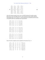
displacements and the corresponding nodal forces of the frame, without the support and
loading conditions. Since each node has three DOFs, the frame has a total of nine nodal
displacements and nine corresponding nodal forces as shown in the figure below.
The nine nodal displacements and the corresponding nodal forces.
It should be emphasized that the nine nodal displacements completely define the
deformation of each member and the entire frame. In the matrix displacement
formulation, we seek to find the matrix equation that links the nine nodal forces to the
nine nodal displacements in the following form:
K
G
∆
G
= F
G
(18)
where K
G
,

∆
G
and F
G
are the global unconstrained stiffness matrix, global nodal
displacement vector, and global nodal force vector, respectively. Eq. 18 in its expanded
form is shown below, which helps identify the nodal displacement and force vectors.
⎥
⎥
⎥

⎥
⎥
⎥
⎥
⎥
⎥
⎥
⎥
⎥
⎦
⎤
⎢
⎢
⎢
⎢
⎢
⎢
⎢
⎢
⎢
⎢
⎢
⎢
⎣
⎡
⎪
⎪
⎪
⎪
⎪

⎪
⎭
⎪
⎪
⎪
⎪
⎪
⎪
⎬
⎫
⎪
⎪
⎪
⎪
⎪
⎪
⎩
⎪
⎪
⎪
⎪
⎪
⎪
⎨
⎧
3
3
3
2
2

2
1
1
1
θ
∆
∆
θ
∆
∆
θ
∆
∆
y
y
x
x
y
x


=
⎪
⎪
⎪
⎪
⎪
⎪
⎭
⎪

⎪
⎪
⎪
⎪
⎪
⎬
⎫
⎪
⎪
⎪
⎪
⎪
⎪
⎩
⎪
⎪
⎪
⎪
⎪
⎪
⎨
⎧
3
3
3
2
2
2
1
1

1
M
F
F
M
F
F
M
F
F
x
x
y
x
y
x

(18)
1
2
3
x
y

∆

x1
θ
1
θ

3
θ
2
1
2
3
x
y
F
x1
M
1
F
y1
F
x3
F
x2
F
y3
F
y2
M
3
M
2
M
ember 1-2
M
ember 2-3

∆

x2
∆

x3

∆

y1

∆

y2
∆

y3
Beam and Frame Analysis: Displacement Method, Part II by S. T. Mau
236
According to the direct stiffness method, the contribution of member 1-2 to the global
stiffness matrix will be at the locations indicated in the above figure, i.e., corresponding
to the DOFs of the first and the second nodes, while the contribution of member 2-3 will
be associated with the DOFs at nodes 2 and 3.
Before we assemble the global stiffness matrix, we need to formulate the member
stiffness matrix.
Member stiffness matrix in local coordinates. For a frame member, both axial and
flexural deformations must be considered. As long as the deflections associated with
these deformations are small relative to the transverse dimension of the member, say
depth of the member, the axial and flexural deformations are independent from each
other; thus allowing us to consider them separately. To characterize the deformations of

a frame member i-j, we need only four independent variables,
∆
x
,
θ
i
,
θ
j
, and
φ
ij
as shown
below.
The four independent deformation configurations and the associated nodal forces.
Each of the four member displacement variables is related to the six nodal displacements
of a member via geometric relations. Instead of deriving these relations mathematically,
then use mathematical transformation to obtain the stiffness matrix, as was done in the
truss formulation, we can establish the stiffness matrix directly by relating the nodal
forces to a nodal displacement, one at a time. We shall deal with the axial displacements
first.
There are two nodal displacements, u
i
and u
j
, related to axial deformation,
∆
x
. We can
easily establish the nodal forces for a given unit nodal displacement, utilizing the nodal

force information in the previous figure. For example, u
i
=1 while other displacements
are zero, corresponds to a negative elongation. As a result, the nodal force at node i is
EA/L, while that at node j is −EA/L. On the other hand, for u
j
=1, the force at node i is
−EA/L, while that at node j is EA/L. These two cases are depicted in the figure below.
∆
x
=1
E
A/L
E
A/L
θ
i
=1
4EK
2EK
6EK/L
6EK/L
θ
j
=1
2EK
4EK
6EK/L
6EK/L
φ

ij
=1
−6EK
−6EK
−12EK/L
−12EK/L
θ
j
=1
∆
x
=1
θ
i
=1
φ
ij
=1
Beam and Frame Analysis: Displacement Method, Part II by S. T. Mau
237
Note we must express the nodal forces in the positive direction of the defined global
coordinates.
Nodal forces associated with a unit nodal displacement.
From the above figure, we can immediately establish the following stiffness relationship.
⎥
⎥
⎥
⎥
⎥
⎦

⎤
⎢
⎢
⎢
⎢
⎢
⎣
⎡
−
−
L
EA
L
EA
L
EA
L
EA
⎭
⎬
⎫
⎩
⎨
⎧
j
i
u
u
=
⎭

⎬
⎫
⎩
⎨
⎧
j
x
i
x
f
f
(19)
Following the same principle, we can establish the flexural relations one at a time as
shown in the figure below.
Nodal forces associated with a unit nodal displacement.
From the above figure we can establish the following flexural stiffness relationship.
−EA/L
E
A/L
E
A/L−EA/L
u
i
=1
u
j
=1
θ
i
=1

4EK
2EK
−6EK/L
6EK/L
θ
j
=1
2EK
4EK
−6EK/L
6EK/L
v
i
=1
−6EK/L
−6EK/L
12EK/L
2
−12EK/L
2
v
j
=1
6EK/L
6EK/L
−12EK/L
2
12EK/L
2
v

i
=0,
θ
i
=1, v
j
=0,
θ
j
=0 v
i
=0,
θ
i
=0, v
j
=0,
θ
j
=1
v
i
=1
,

θ
i
=0
,
v

j
=0
,

θ
j
=0 v
i
=0
,

θ
i
=0
,
v
j
=1
,

θ
j
=0
u
i
=1
,
u
j
=0 u

i
=0
,
u
j
=1
Beam and Frame Analysis: Displacement Method, Part II by S. T. Mau
238
⎥
⎥
⎥
⎥
⎥
⎥
⎥
⎥
⎥
⎦
⎤
⎢
⎢
⎢
⎢
⎢
⎢
⎢
⎢
⎢
⎣
⎡

−
−
−
−−−
EK
L
EK
EK
L
EK
L
EK
2
L
EK
L
EK
2
L
EK
EK
L
EK
EK
L
EK
L
EK
2
L

EK
L
EK
2
L
EK
4
6
2
6
612612
2
6
4
6
612612
⎪
⎪
⎭
⎪
⎪
⎬
⎫
⎪
⎪
⎩
⎪
⎪
⎨
⎧

j
j
i
i
v
v
θ
θ
=
⎪
⎪
⎭
⎪
⎪
⎬
⎫
⎪
⎪
⎩
⎪
⎪
⎨
⎧
j
yj
i
yi
M
f
M

f
(20)
Eq. 20 is the member stiffness equation of a flexural member, while Eq. 19 is that of a
axial member. The stiffness equation for a frame member is obtained by the merge of the
two equations.
⎥
⎥
⎥
⎥
⎥
⎥
⎥
⎥
⎥
⎥
⎥
⎥
⎥
⎥
⎥
⎥
⎥
⎦
⎤
⎢
⎢
⎢
⎢
⎢
⎢

⎢
⎢
⎢
⎢
⎢
⎢
⎢
⎢
⎢
⎢
⎢
⎣
⎡
−
−
−
−
−−−
−
EK
L
EK
EK
L
EK
L
EK
L
EK
L

EK
L
EK
L
EA
L
EA
EK
L
EK
EK
L
EK
L
EK
L
EK
L
EK
L
EK
L
EA
L
EA
4
6
2
6
612612

2
6
4
6
612612
00
00
0000
00
00
0000
22
22
⎪
⎪
⎪
⎪
⎪
⎪
⎪
⎭
⎪
⎪
⎪
⎪
⎪
⎪
⎪
⎬
⎫

⎪
⎪
⎪
⎪
⎪
⎪
⎪
⎩
⎪
⎪
⎪
⎪
⎪
⎪
⎪
⎨
⎧
j
j
j
i
i
i
v
u
v
u
θ
θ
=

⎪
⎪
⎪
⎪
⎪
⎪
⎪
⎭
⎪
⎪
⎪
⎪
⎪
⎪
⎪
⎬
⎫
⎪
⎪
⎪
⎪
⎪
⎪
⎪
⎩
⎪
⎪
⎪
⎪
⎪

⎪
⎪
⎨
⎧
j
yj
xj
i
yi
xi
M
f
f
M
f
f
(21)
Eq. 21 is the member stiffness equation in local coordinates and the six-by-six matrix at
the LHS is the member stiffness matrix in local coordinates. Eq. 21 can be expressed in
matrix symbols as
k
L
δ
L
= f
L
(21)
Member stiffness matrix in global coordinates. In the formulation of equilibrium
equations at each of the three nodes of the frame, we must use a common set of
coordinate system so that the forces and moments are expressed in the same system and

can be added directly. The common system is the global coordinate system which may
not coincide with the local system of a member. For a typical orientation of a member as
shown, we seek the member stiffness equation in the global coordinates:
k
G
δ
G
= f
G
(22)
Beam and Frame Analysis: Displacement Method, Part II by S. T. Mau
239
We shall derive Eq. 22 using Eq. 21 and the formulas that relate the nodal displacement
vector,
δ
L
, and the nodal force vector, f
L
to their global counterparts,
δ
G
and f
G
,
respectively.
Nodal displacements in local and global coordinates.
Nodal forces in local and global coordinates.
Vector de-composition.
From the vector de-composition, we can express the nodal displacements in local
coordinates in terms of the nodal displacements in global coordinates.

∆
xj
= (Cos
β
) u
j
– (Sin
β
) v
j
β
u
j
u
i
v
j
v
i

∆
xj

∆
yj

∆
xi

∆

yi
β
f

xj
F
xj


F
xi
F
yi
θ
j
θ
j
θ
i
θ
i
ii
j
j
j
j
i
i
f

yj
f

xi
f

yi


F
yj
M
j
M
j
M
i
M
i

∆
xj

∆
yj
β
u
j

∆

xj

∆
yj
β
v
j
Beam and Frame Analysis: Displacement Method, Part II by S. T. Mau
240
∆
yj
= (Sin
β
) u
j
+ (Cos
β
) v
j
θ
j
=
θ
j
Identical formulas can be obtained for node i. The same transformation also applies to the
transformation of nodal forces. We can put all the transformation formulas in matrix
form, denoting Cos
β
and Sin
β

by C and S, respectively.
⎪
⎭
⎪
⎬
⎫
⎪
⎩
⎪
⎨
⎧
i
yi
xi
θ
∆
∆
=
⎥
⎥
⎥
⎦
⎤
⎢
⎢
⎢
⎣
⎡
100
0

0
CS
S-C
⎪
⎭
⎪
⎬
⎫
⎪
⎩
⎪
⎨
⎧
i
i
i
v
u
θ
or
∆
iG
=
τ ∆
iL
⎪
⎭
⎪
⎬
⎫

⎪
⎩
⎪
⎨
⎧
j
yj
xj
θ
∆
∆
=
⎥
⎥
⎥
⎦
⎤
⎢
⎢
⎢
⎣
⎡
100
0
0
CS
S-C
⎪
⎭
⎪

⎬
⎫
⎪
⎩
⎪
⎨
⎧
j
j
j
v
u
θ
or
∆
jG
=
τ ∆
jL
⎪
⎭
⎪
⎬
⎫
⎪
⎩
⎪
⎨
⎧
i

yi
xi
M
F
F
=
⎥
⎥
⎥
⎦
⎤
⎢
⎢
⎢
⎣
⎡
100
0
0
CS
S-C
⎪
⎭
⎪
⎬
⎫
⎪
⎩
⎪
⎨

⎧
i
yi
xi
M
f
f
or

f
iG
=
τ
f
iL
⎪
⎭
⎪
⎬
⎫
⎪
⎩
⎪
⎨
⎧
j
yj
xj
M
F

F
=
⎥
⎥
⎥
⎦
⎤
⎢
⎢
⎢
⎣
⎡
100
0
0
CS
S-C
⎪
⎭
⎪
⎬
⎫
⎪
⎩
⎪
⎨
⎧
j
yj
xj

M
f
f
or

f
jG
=
τ
f
jL
The transformation matrix
τ
has a unique feature. i.e., its inverse is equal to its transpose
matrix.
τ
−1
=
τ
T
Matrices satisfy the above equation are called orthonormal matrices. Because of this
unique feature of orthonormal matrices, we can easily write the inverse relationship for
all the above four equations. We need, however, only the inverse formulas for nodal
displacements:
⎪
⎭
⎪
⎬
⎫
⎪

⎩
⎪
⎨
⎧
i
i
i
v
u
θ
=
⎥
⎥
⎥
⎦
⎤
⎢
⎢
⎢
⎣
⎡
100
0
0
CS-
SC
⎪
⎭
⎪
⎬

⎫
⎪
⎩
⎪
⎨
⎧
i
yi
xi
θ
∆
∆
or
∆
∆
iL
=
τ
T
∆
iG
Beam and Frame Analysis: Displacement Method, Part II by S. T. Mau
241
⎪
⎭
⎪
⎬
⎫
⎪
⎩

⎪
⎨
⎧
j
j
j
v
u
θ
=
⎥
⎥
⎥
⎦
⎤
⎢
⎢
⎢
⎣
⎡
100
0
0
CS-
SC
⎪
⎭
⎪
⎬
⎫

⎪
⎩
⎪
⎨
⎧
j
yj
xj
θ
∆
∆
or
∆
∆
jL
=
τ
T
∆
jG
The nodal displacement vector and force vector of a member,
δ
G
,
δ
L
, f
G
and f
L

, are the
collections of the displacement and force vectors of node i and node j:
δ
G
=
⎭
⎬
⎫
⎩
⎨
⎧
jG
iG
∆
∆
δ
L
=
⎭
⎬
⎫
⎩
⎨
⎧
jL
iL
∆
∆
f
G

=
⎭
⎬
⎫
⎩
⎨
⎧
jG
iG
f
f
f
L
=
⎭
⎬
⎫
⎩
⎨
⎧
jL
iL
f
f
To arrive at Eq. 22, we begin with
f
G
=
⎭
⎬

⎫
⎩
⎨
⎧
jG
iG
f
f
=
⎥
⎦
⎤
⎢
⎣
⎡
τ
τ
0
0
⎭
⎬
⎫
⎩
⎨
⎧
jL
iL
f
f
=

Γ
f
L
(23)
where
Γ
=
⎥
⎦
⎤
⎢
⎣
⎡
τ
τ
0
0
(24)
From Eq. 21, and the transformation formulas for nodal displacements, we obtain
f
L
= k
L
δ
L
= k
L

⎭
⎬

⎫
⎩
⎨
⎧
jL
iL
∆
∆
= k
L
⎥
⎥
⎦
⎤
⎢
⎢
⎣
⎡
T
T
τ
τ
0
0
⎭
⎬
⎫
⎩
⎨
⎧

jG
iG
∆
∆
= k
L

Γ
T
δ
G
(25)
Combining Eq. 25 with Eq. 23, we have
f
G
=
Γ
f
L
=
Γ
k
L

Γ
T
δ
G
(22)
which is in the form of Eq. 22, with

k
G
=
Γ
k
L

Γ
T

(26)
Eq. 26 is the transformation formula of the member stiffness matrix. The expanded form
of the member stiffness matrix in its explicit form in global coordinates, k
G
, appears as a
six-by-six matrix:
Beam and Frame Analysis: Displacement Method, Part II by S. T. Mau
242
k
G
=
⎥
⎥
⎥
⎥
⎥
⎥
⎥
⎥
⎥

⎥
⎥
⎥
⎥
⎥
⎥
⎥
⎥
⎦
⎤
⎢
⎢
⎢
⎢
⎢
⎢
⎢
⎢
⎢
⎢
⎢
⎢
⎢
⎢
⎢
⎢
⎢
⎣
⎡
−

+−−−−−
−−+−−−−−
−−
−−−−−−+−
−−−−−+
EK
L
EK
C
L
EK
S-EK
L
EK
C
L
EK
S
L
EK
C
L
EK
C
L
EA
S
L
EK
L

EA
CS
L
EK
C
L
EK
C
L
EA
S
L
EK
L
EA
CS
L
EK
S
L
EK
L
EA
CS
L
EK
S
L
EA
C

L
EK
S
L
EK
L
EA
CS
L
EK
S
L
EA
C
EK
L
EK
C
L
EK
SEK
L
EK
C
L
EK
S
L
EK
C

L
EK
C
L
EA
S
L
EK
L
EA
CS
L
EK
C
L
EK
C
L
EA
S
L
EK
L
EA
CS
L
EK
S
L
EK

L
EA
CS
L
EK
S
L
EA
C
L
EK
S
L
EK
L
EA
CS
L
EK
S
L
EA
C
4
66
2
66
612
)
12

(
612
)
12
(
6
)
12
(
126
)
12
(
12
2
66
4
66
612
)
12
(
612
)
12
(
6
)
12
(

126
)
12
(
12
2
22
22
22
2
22
22
22
22
2
22
22
22
2
22
22
22
22
(26)
The corresponding nodal displacement and force vectors, in their explicit forms, are
δ
G
=
⎪
⎪

⎪
⎪
⎭
⎪
⎪
⎪
⎪
⎬
⎫
⎪
⎪
⎪
⎪
⎩
⎪
⎪
⎪
⎪
⎨
⎧
j




yj
xj
i
y
xi

θ
∆
∆
θ
∆
∆
i
and f
G
=
⎪
⎪
⎪
⎪
⎭
⎪
⎪
⎪
⎪
⎬
⎫
⎪
⎪
⎪
⎪
⎩
⎪
⎪
⎪
⎪

⎨
⎧
j
yj
xj
i
yi
xi
M
F
F
M
F
F
(27)
Unconstrained global equilibrium equation. The member stiffness matrices are
assembled into a matrix equilibrium equation, which are formulated from the three
equilibrium equations at each node: two force equilibrium and one moment equilibrium
equations. The method of assembling is according to the direct stiffness method outlined
in the matrix analysis of trusses. For the present case, there are nine equations from the
three nodes as indicated in Eq. 18.
Constrained global equilibrium equation. Out of the nine nodal displacements, six are
constrained to be zero because of support conditions at nodes 1 and 3. There are only
three unknown nodal displacements:
∆
x2
,
∆
y2
, and

θ
2
. On the other hand, out of the nine
nodal forces, only three are given: F
x2
= 2 kN, F
y2
=0, and M
2
= -2 kN-m; the other six are
unknown reactions at the supports. Once we specify all the known quantities, the global
equilibrium equation appears in the following form:
Beam and Frame Analysis: Displacement Method, Part II by S. T. Mau
243
⎥
⎥
⎥
⎥
⎥
⎥
⎥
⎥
⎥
⎥
⎥
⎥
⎦
⎤
⎢
⎢

⎢
⎢
⎢
⎢
⎢
⎢
⎢
⎢
⎢
⎢
⎣
⎡
999897969594
898887868584
797877767574
696867666564636261
595857565554535251
494847464544434241
363534333231
262524232221
161514131211
000
000
000


000
000
000
KKKKKK

KKKKKK
KKKKKK
KKKKKKKKK
KKKKKKKKK
KKKKKKKKK
KKKKKK
KKKKKK
KKKKKK
⎪
⎪
⎪
⎪
⎪
⎪
⎭
⎪
⎪
⎪
⎪
⎪
⎪
⎬
⎫
⎪
⎪
⎪
⎪
⎪
⎪
⎩

⎪
⎪
⎪
⎪
⎪
⎪
⎨
⎧
0
0
0
0
0
0
2
2
2
θ
∆
∆
y
x
=
⎪
⎪
⎪
⎪
⎪
⎪
⎭

⎪
⎪
⎪
⎪
⎪
⎪
⎬
⎫
⎪
⎪
⎪
⎪
⎪
⎪
⎩
⎪
⎪
⎪
⎪
⎪
⎪
⎨
⎧
3
3
3
1
1
1
2-

0
2
M
F
F
M
F
F
x
x
y
x

(18)
The solution of Eq. 18 comes in two steps. The first step is to solve for only the three
displacement unknowns using the three equations in the fourth to sixth rows of Eq. 18.
⎥
⎥
⎥
⎦
⎤
⎢
⎢
⎢
⎣
⎡
666564
565554
464544
KKK

KKK
KKK
⎪
⎭
⎪
⎬
⎫
⎪
⎩
⎪
⎨
⎧
2
2
2
θ
∆
∆
y
x
=
⎪
⎭
⎪
⎬
⎫
⎪
⎩
⎪
⎨

⎧
2-
0
2
(28)
Once the nodal displacements are known, we can carry out the second step by
substituting back to Eq. 18 all the nodal displacements and computing the six other nodal
forces, which are the support reaction forces. We also need to find the member-end
forces through Eq. 21, which requires the determination of nodal displacements in local
coordinates.
We shall demonstrate the above procedures through a numerical example.
Example 16. Find the nodal displacements, support reactions, and member-end forces of
all members of the frame shown. E= 200 GPa, A=20,000 mm
2
, and I= 300x10
6
mm
4
for
the two members.
Example problem.
1
2
3
2 kN
2 kN-m
x
y
4 m
2 m

Beam and Frame Analysis: Displacement Method, Part II by S. T. Mau
244
Solution. We will carry out a step-by-step solution procedure for the problems.
(1) Number the nodes and members and define the nodal coordinates
Nodal Coordinates
Node x (m) y (m)
100
204
324
(2) Define member property, starting and end nodes and compute member data
Member Input Data
Member
Starting
Node
End
Node
E
(GPa)
I
(mm
4
)
A
(mm
2
)
1 1 2 200 3x10
8
2x10
4

2 2 3 200 3x10
8
2x10
4
Computed Data
Member
∆
X
(m)
∆
Y
(m)
L
(m)
CS
EI
(kN-m
2
)
EA
(kN)
1 0 4 4 0.0 1.0 6x10
4
4x10
9
2 2 0 2 1.0 0.0 6x10
4
4x10
9
In computing the member data, the following formulas were used:

L=
22
)()(
ii
yyxx
jj
−+−
C= Cos
β
=
L
xx
ij
)( −
=
L
x
∆
S= Sin
β
=
L
yy
ij
)( −
=
L
y
∆
(3) Compute member stiffness matrices in global coordinates: Eq. 26

Member 1:
Beam and Frame Analysis: Displacement Method, Part II by S. T. Mau
245

(k
G
)
1
=
⎥
⎥
⎥
⎥
⎥
⎥
⎥
⎥
⎦
⎤
⎢
⎢
⎢
⎢
⎢
⎢
⎢
⎢
⎣
⎡
60,000022,500-30,000022,500

01x10001x10-0
22,500-011,25022,500-011,250-
30,0000 22,500-60,000022,500
0 1x10-001x100
22,500011,250-22,500011,250
99
99
Member 2:
(k
G
)
2
=
⎥
⎥
⎥
⎥
⎥
⎥
⎥
⎥
⎦
⎤
⎢
⎢
⎢
⎢
⎢
⎢
⎢

⎢
⎣
⎡
44
99
44
99
12x1090,00006x1090,000-0
90,00090,000-090,00090,000-0
002x10002x10-
6x1090,000012x1090,000-0
90,000-90,000-090,000-90,0000
002x10-002x10
(4) Assemble the unconstrained global stiffness matrix
In order to use the direct stiffness method to assemble the global stiffness matrix, we
need the following table which gives the global DOF number corresponding to each local
DOF of each member. This table is generated using the member data given in the table in
subsection (2), namely the starting and end nodes data.
Global DOF Number for Each Member
Global DOF Number
for Member
Local
Nodal DOF
Number
12
11 4
22 5
Starting
Node
i

33 6
44 7
55 8
End
Node
j
66 9

Armed with this table we can easily direct the member stiffness components to the right
location in the global stiffness matrix. For example, the (2,3) component of (k
G
)
2
will be
added to the (5,6) component of the global stiffness matrix. The unconstrained global
stiffness matrix is obtained after the assembling is done.
Beam and Frame Analysis: Displacement Method, Part II by S. T. Mau
246
K
G
=
⎥
⎥
⎥
⎥
⎥
⎥
⎥
⎥
⎥

⎥
⎥
⎥
⎥
⎥
⎦
⎤
⎢
⎢
⎢
⎢
⎢
⎢
⎢
⎢
⎢
⎢
⎢
⎢
⎢
⎢
⎣
⎡
−
−−
−
−−
−−−
−−−−
−

−
−
000,120000,900000,60000,900000
90,000000,900000,90000,900000
00
9
10x200
9
10x2000
60,00090,0000180,00090,00022,50030,000022,500
90,00090,000090,000
9
10x100
9
10x10
00
9
10x222,5000
9
10x2500,
220250,11
000000,300500,22000,600500,22
0000
9
10x100
9
10x10
000500,220250,11500,220250,11
(5) Constrained global stiffness equation and its solution
Once the support and loading conditions are incorporated into the stiffness equations we

obtain the constrained global stiffness equation as given in Eq. 18, which is reproduced
below for easy reference, with the stiffness matrix shown in the above equation.
⎥
⎥
⎥
⎥
⎥
⎥
⎥
⎥
⎥
⎥
⎥
⎥
⎦
⎤
⎢
⎢
⎢
⎢
⎢
⎢
⎢
⎢
⎢
⎢
⎢
⎢
⎣
⎡

999897969594
898887868584
797877767574
696867666564636261
595857565554535251
494847464544434241
363534333231
262524232221
161514131211
000
000
000


000
000
000
KKKKKK
KKKKKK
KKKKKK
KKKKKKKKK
KKKKKKKKK
KKKKKKKKK
KKKKKK
KKKKKK
KKKKKK
⎪
⎪
⎪
⎪

⎪
⎪
⎭
⎪
⎪
⎪
⎪
⎪
⎪
⎬
⎫
⎪
⎪
⎪
⎪
⎪
⎪
⎩
⎪
⎪
⎪
⎪
⎪
⎪
⎨
⎧
0
0
0
0

0
0
2
2
2
θ
∆
∆
y
x
=
⎪
⎪
⎪
⎪
⎪
⎪
⎭
⎪
⎪
⎪
⎪
⎪
⎪
⎬
⎫
⎪
⎪
⎪
⎪

⎪
⎪
⎩
⎪
⎪
⎪
⎪
⎪
⎪
⎨
⎧
3
3
3
1
1
1
2-
0
2
M
F
F
M
F
F
x
x
y
x

(18)
For the three displacement unknowns the following three equations taking from the
fourth to sixth rows of the unconstrained global stiffness equation are the governing
equations.

⎥
⎥
⎥
⎦
⎤
⎢
⎢
⎢
⎣
⎡
180,00090,000-22,500-
90,000-1x100
22,500-02x10
9
9
⎪
⎭
⎪
⎬
⎫
⎪
⎩
⎪
⎨

⎧
2
2
2
θ
∆
∆
y
x
=
⎪
⎭
⎪
⎬
⎫
⎪
⎩
⎪
⎨
⎧
2-
0
2
(28)
Beam and Frame Analysis: Displacement Method, Part II by S. T. Mau
247
The solutions are:
∆
x2
=0.875x10

-9

m,
∆
y2
=1x10
-9
m, and
θ
2
=1.11x10
-5
rad. Upon
substituting the nodal displacements into Eq. 18, we obtain the nodal forces, which are
support reactions:
⎪
⎪
⎭
⎪
⎪
⎬
⎫
⎪
⎪
⎩
⎪
⎪
⎨
⎧
1

1
1
M
F
F
y
x
=
⎪
⎪
⎭
⎪
⎪
⎬
⎫
⎪
⎪
⎩
⎪
⎪
⎨
⎧
−
m-kN 0.33-
kN 1.00
kN 25.0
and
⎪
⎪
⎭

⎪
⎪
⎬
⎫
⎪
⎪
⎩
⎪
⎪
⎨
⎧
3
3
3
M
F
F
y
x
=
⎪
⎪
⎭
⎪
⎪
⎬
⎫
⎪
⎪
⎩

⎪
⎪
⎨
⎧
−
−
−
m-kN 0.67
kN 1.00
kN 75.1
(6) Compute member nodal forces in local coordinates
The member nodal forces in local coordinates are needed to draw shear and moment
diagrams and are obtained using Eq. 21. The nodal displacements in local coordinates in
Eq. 21 are computed using the transformation formula
⎪
⎭
⎪
⎬
⎫
⎪
⎩
⎪
⎨
⎧
i
i
i
v
u
θ

=
⎥
⎥
⎥
⎦
⎤
⎢
⎢
⎢
⎣
⎡
100
0
0
CS-
SC
⎪
⎭
⎪
⎬
⎫
⎪
⎩
⎪
⎨
⎧
i
yi
xi
θ

∆
∆
or
∆
∆
iL
=
τ
T
∆
iG
The results are presented in the following reaction, shear, moment and deflection
diagrams.

Reaction, shear, moment, and deflection diagrams.
1
2
3
2 kN
2 kN-m
0.67 kN-m
0.33 kN-m
0.25 kN
1 kN
1 kN
0.25 kN
1 kN
0.33 kN-m
0.67 kN-m
0.67 kN-m

1.33 kN-m
I
nflection point
Beam and Frame Analysis: Displacement Method, Part II by S. T. Mau
248
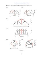
Problem 3. Prepare the input data set needed for the matrix solution of the frame shown.
Begin with the numbering of nodes and members. E= 200 GPa, A=20,000 mm
2
, and I=
300x10
6
mm
4
for the three members.
Problem 3.
2 kN
5 kN-m
4 m
2 m
3 m
249
Influence Lines
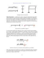
1. What is Influence Line?
In structural design, it is often necessary to find out what the expected maximum quantity
is for a selected design parameter, such as deflection at a particular point, a particular
stress at a section, etc. The answer obviously depends on how the load is applied. The
designer must apply the load in such a way that the maximum quantity for the selected
parameter is obtained. The load could be concentrated loads, single or multiple, or
distributed loads over a specified length or area. For a single concentrated load, it is
often possible to guess where the load should be placed in order to result in a maximum

quantity for a sectional moment of a beam, for example. For multiple-load, it is less likely
that a correct answer can come from a guess.
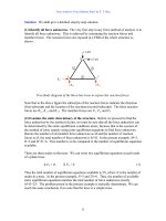
Take the beam shown as an example. We are interested in finding the maximum moment
of section c for a concentrated vertical load of a unit magnitude. Intuition tells us that we
should place the vertical load directly at c. This guess turns out to be the correct answer.
If, however, we have two unit loads, one tenth of the span, L, apart from each other. We
have at least two possibilities as shown and intuition cannot tell us which will produce
the maximum moment at c.
A beam with two loading possibilities to produce maximum moment at c.
A systematic way of finding the maximum quantity of a parameter is the influence line
approach. The concept is simple: compute the response of the targeted parameter to a
unit load at “every” location and plot the result against the location of the unit load. The
x-y plot is the influence line. For a single concentrated load, the peak of the influence
line gives the location of the load. The maximum quantity is then the product of the
influence line value at the peak and the magnitude of the load. For multiple-load, the
maximum is the summation of each load computed in the same way as the single load.
L
/2
L
/2
ac
b
a
c
b
ac
b
0.1L
L
/2

L
/2
0.1L
L
/2
L
/2
Influence Lines by S. T. Mau
250
The shape of the influence line usually reveals the locations for the multiple-load. For
distributed load, the maximum is achieved by placing the load where the area under the
influence line is the greatest.
To construct the influence line, it is not necessary to analyze the structure for every
location of the unit load, although it can be done with a computer program for any
number of selected locations. We shall introduce the analytical way of constructing
influence lines.
2. Beam Influence Lines
Consider the beam shown below. We wish to construct the influence lines for R
b
, V
c
and
M
c
.
Influence lines for R
b
, V
c
and M

c
are to be constructed.
The problem can be defined as finding R
b
, V
c
and M
c
as a function of x, the location of the
unit load shown below.
Location of the unit load is the variable.
We recognize that the three parameters R
b
, V
c
and M
c
are all related to the reactions at a
and b. Thus, we solve for R
a
and R
b
first.
FBD to solve for R
a
and R
b
.
ac
b

1
x
ac
b
1
x
R
a
R
b
L
/2
L
/2
ac
b
Influence Lines by S. T. Mau
251
ΣM
b
=0 R
a
= (L-x)/L ΣM
a
=0 R
b
= x/L
Having obtained R
a
and R

b
as linear functions of the location of the unit load, we can plot
the functions as shown below with the horizontal coordinate being x. These influence
lines can be used to find influence lines of R
b
, V
c
and M
c
.
Influence lines for R
a
and R
b
.
For V
c
and M
c
, we need to solve for them using appropriate free-body-diagrams.
FBDs to solve for V
c
and M
c
.
The above FBDs are selected so that we do not have to include the unit load in the
equilibrium equations. Consequently, the left FBD is valid for the unit load being located
to the right of section c (x>L/2 ) and the right FBD is for the unit load located to the left
of the section(x<L/2 ). From each FBD, we can obtain the expressions of V
c

and M
c
as
functions of R
a
and R
b
.
Left FBD: Valid for x>L/2 Right FBD: Valid For x<L/2
V
c
= R
a
V
c
= −R
b
M
c
= R
a
L/2 M
c
= R
b
L/2
Using the influence lines of R
a
and R
b

we can construct the influence lines of V
c
and M
c
by cut-and-paste and adjusting for the factors L/2 and the negative sign.
1
1
R
a
R
b
M
c
M
c
V
cV
c
R
a
R
b
F
or x>L/2
F
or x<L/2
Influence Lines by S. T. Mau
252
Use the influence lines of R
a

and R
b
to construct the influence lines of V
c
and M
c
.
Müller-Breslau Principle. The above process is laborious but serves the purpose of
understanding the analytical way of finding solutions for influence lines. For beam
influence lines, a quicker way is to apply the Müller-Breslau Principle, which is derived
from the virtual work principle. Consider the FBD and the same FBD with a virtual
displacement shown below.
FBDs of a beam and a virtually displaced beam.
1
1
R
a
R
b
1/2
1/2
V
c
L
/4
M
c
ac
b
1

x
R
a
R
b
a
c
b
1
x
R
a
R
b
1
y
Influence Lines by S. T. Mau
253
The virtual work principle states that for an equilibrium system, the work done by all
forces upon a set of virtual dispalcment is zero. Since the only forces having a
corresponding virtual displacement are R
a
and the unit load, we obtain:
(1) R
a
+ (−y) 1=0 R
a
= y
The abovo result indicates that the influence line of R
a

is numerically equal to
the virtual displacement of the beam, when the virtual displacement is constructed with a
unit displacement at R
a
and no displacements at any forces except the unit load.
Consider one more set of virtual displacement of the beam aimmed at exposing the
sectional force V
c
.
Beam and associated virtual displacement for V
c
.
Application of the virtual work principle leads to:
(1) V
c
+ (y) 1=0 V
c
= − y
where y is positive if upward and negative if downward.
Another set of virtual displacement designed for solving M
c
is shown below.
ac
b
x
a
x
b
1/2
1/2

M
c
V
c
M
c
V
c
y
1
1
Influence Lines by S. T. Mau
254
Virtual displacement for solving M
c
.
The application of the virtual work principle leads to
(1) M
c
+ (-y) 1=0 M
c
= y
From the above results, we can state that a properly constructed virtual displacement
which does not incur any workdone by any force other then the force of interest and the
unit load gives the shape of the influence line for the force of interest. This is called the
Müller-Breslau Principle.
The step-by-step process of applying the Müller-Breslau Principle can be summarized as
follows:
(1) Expose the quantity of interest by a cut (or remove a support).
(2) Impose a virtual displacement such that

(a) at the cut there is a unit displacement (or rotation).
(b) the quantity of interest produces a positive work.
(c) no other internal force produces any work.
(3) The resulting displacement shape is the desired influence line.
Example 1. Construct the influence lines for R
a
, R
b
, V
c
, M
c
, V
d
, and M
d
of the beam
shown.
Beam with an overhang.
Solution. We shall use the Müller-Breslau Principle to construct the influence lines. It is
a try-and-error process to make sure the condition that no other forces produce any work
is satisfied.
a
x
b
M
c
V
c
M

c
V
c
y
1
1
a
b
c
d