Physical Processes in Earth and Environmental Sciences Phần 2 ppt
Bạn đang xem bản rút gọn của tài liệu. Xem và tải ngay bản đầy đủ của tài liệu tại đây (1.81 MB, 34 trang )
20 Chapter 2
4 Magma has small but important fractions of pressurized
dissolved gases, including water vapor.
5 River water contains suspended solids, while the atmos-
phere carries dust particles and liquid aerosols.
6 Seawater has c.3 percent by weight of dissolved salts and
also suspensions of particulate organic matter.
Solid Earth substances may break or flow:
1 Ice fragments when struck, yet deformation of boreholes
drilled to the base of glaciers also shows that the ice there
flows, while cracking along crevasses at the surface.
2 Earth’s mantle imaged by rapidly transmitted seismic
waves behaves as a solid mass of crystalline silicate minerals.
Yet there is ample evidence that in the longer term
(Ͼ10
3
years) it flows, convecting most of Earth’s internal
heat production as it does so. Even the rigid lower crust is
thought to flow at depth, given the right temperature and
water content.
2.1.5 Timescales of
in situ
reaction
The lesson from the last of the above examples is that we
must appreciate characteristic timescales of reaction of
Earth materials to imposed forces and be careful to relate
state behavior to the precise conditions of temperature and
pressure where the materials are found in situ.
2.2 Thermal matters
2.2.1 Heat and temperature
Heat is a more abstract and less commonsense notion than
temperature, the use of the two terms in everyday speech
being almost synonymous. We measure temperature with
some form of heat sensor or thermometer. It is a measure
of the energy resulting from random molecular motions in
any substance. It is directly proportional to the mean
kinetic energy, that is, mean product of mass times velocity
squared (Section 3.3), of molecules. Heat on the other
hand is a measure of the total thermal energy, depending
again on the kinetic energy of molecules, and also on the
number of molecules present in any substance.
It is through specific heat, c, that we can relate temperature
and heat of any substance. Specific heat is a finite capacity,
sometimes referred to as specific heat capacity, in that it is a
measure of how much heat is required to raise the temper-
ature of a unit mass (1 kg) of any substance by unit Kelvin
(K ϭЊC ϩ 273). It is thus also a storage indicator – since
only a certain amount of heat is required to raise tempera-
ture between given limits, it follows that only this amount
of heat can be stored. In Box 2.1, notice the extremely
high storage capacity of water, compared to the gaseous
atmosphere or rock.
Temperature change induces internal changes to
any substance and also external changes to surrounding
environments, for example,
1 Molten magma cools on eruption at Earth’s surface, turn-
ing into lava; this in turn slowly crystallizes into rock.
2 Glacier ice in icebergs takes in heat from contact with
the ocean, expands, and melts. The liquid sinks or floats
depending upon the density of surrounding seawater.
3 Water vapor in a descending air mass condenses and
heat is given out to the surrounding atmospheric flow.
In each case temperature change signifies internal energy
change. Changes of state between solid, liquid, and gas
require major energy transfers, expressed as latent heats
(Box 2.1). We shall further investigate the world of ther-
modynamics and its relation to mechanics later in this book
(Section 3.4).
Substances subject to changed temperature also change
volume, and therefore density; they exhibit the phenome-
non of thermal expansion or contraction (Box 2.1). This
arises as constituent atoms and molecules vibrate or travel
around more or less rapidly, and any free electrons flow
around more or less easily. If changes in volume affect only
discrete parts of a body, then thermal stresses are set up
that must be resisted by other stresses failing which a net
force results. Temperature change can thus induce motion
or change in the rate of motion. Stationary air or water
when heated or cooled may move. Molten rock may move
through solid rock. A substance already moving steadily
may accelerate or decelerate if its temperature is forced to
change. But we need to consider the complicating fact that
substances (particularly the flow of fluids) also change in
their resistance to motion, through the properties of vis-
cosity and turbulence, as their temperatures change. We
investigate the forces set up by contrasting densities later
in this book (e.g. Sections 2.17, 4.6, 4.12, and 4.20).
2.2.2 Where does heat energy come from?
There are two sources for the heat energy supplied to
Earth (Fig. 2.4). Both are ultimately due to nuclear reac-
tions. The external source is thermonuclear reactions in
the Sun. These produce an almost steady radiance of
shortwave energy (sunlight is the visible portion), the
LEED-Ch-02.qxd 11/26/05 12:34 Page 20
Matters of state and motion 21
Specific heat capacities, c
p
, units
of J kg
–1
K
–1
, at standard T and P.
Air 1,006
Water vapor (100°C) 2,020
Water 4,182
Seawater 3,900
Olive oil 1,970
Iron 106
Copper 385
Aluminum 913
Silica fiber 788
Carbon (graphite) 710
Mantle rock (olivine) 840
Limestone 880
Coefficients (multiply by 10
–6
) of
linear thermal expansion, a
l
, units
of K
–1
at standard T and P.
Iron 12
Copper 17
Aluminum 23
Silica fiber 0.4
Carbon (graphite) 7.9
Crustal rock (to 373 K) 7–10
Coefficients (multiply by 10
–4
) of
cubical thermal expansion, a
v
, units
of K
–1
at standard T and P.
Water 2.1
Olive Oil 7.0
Crustal rock 0.2–0.3
Thermal conductivity, l, units of
W m
–1
K
–1
at standard T and P.
Air 0.0241
Water 0.591
Olive oil 0.170
Iron 80
Copper 385
Aluminum 201
Silica fiber 9.2
Carbon (graphite) 5
Mantle rock (olivine) 3–4.5
Limestone 2–3.4
Heat flow required for fusion, L
f
,
units of kJ kg
–1
. Sometimes termed latent
heat of fusion, more correctly it is the specific
enthalpy change on fusion (see Section 3.4).
Ice 335
Mg Olivine 871
Na Feldspar 216
Basalt 308
Heat flow required for vaporization, L
v
,
units of kJ kg
–1
. Sometimes termed latent
heat of vaporization, more correctly it is the
specific enthalpy change on vaporization
(see Section 3.4).
water to water vapor
(and vice versa) 2,260
Heat flow produced by crystallization,
(multiply by 10
4
) units of J kg
–1
.
Basalt magma
to basalt 40
Water to ice 32
Thermal Diffusivity, k, units m
2
s
–1
x 10
–6
at
standard T and P.
Air 21.5
Water 0.143
Mantle rock 1.1
Thermal diffusivity indicates the rate of dissemination
of heat with time. It is the ratio of rate of passage of
heat energy (conductivity) to heat energy storage
capacity (specific heat per unit volume) of any material
Specific Heat Capacity , c
p
, c
v
, is the amount of heat
required to raise the temperature of 1 kg of substance
by 1 K . Subscripts refer to constant volume or pressure
Thermal Conductivity is the rate of flow of heat
through unit area in unit time
Box 2.1 Some thermal definitions and properties of earth materials
LEED-Ch-02.qxd 11/26/05 12:34 Page 21
22 Chapter 2
average magnitude of which on an imaginary unit surface
placed at the uppermost surface of Earth’s atmosphere
facing the sun is now approximately 1,367 W m
Ϫ2
. This solar
constant is the result of a luminosity which varies by
>0.3 percent during sunspot cycles, possibly more during
mysterious periods of negligible sunspots like the Maunder
Minimum (300–370 years
BP) coincident with the Little Ice
Age. At any point on Earth’s surface, seasonal variations in
received radiation occur due to planetary tilt and elliptical
orbit, with longer term variations up to 1 percent due to the
Croll–Milankovitch effect (Section 6.1).
Internal heat energy comes from two sources. A minority,
about 20 percent, comes from the “fossil” heat of the
molten outer core. The remainder comes from the radioac-
tive decay of elemental isotopes like
238
U and
40
K locked
up in rock minerals, especially low density granite-type
rocks of the Earth’s crust where such elements have been
concentrated over geological time. However, the total
mass of such isotopes has continued to decrease since the
origin of the Earth’s mantle and crust, so that the mean
internal outward heat flux has also decreased with time.
Today, the mean flux of heat issuing from interior Earth is
around 65 mW m
Ϫ2
(Fig. 2.4), though there are areas of
active volcanoes and geothermally active areas where the
flux is very much greater. The mean flux outward is thus
only some 4.8 и 10
Ϫ5
of the solar constant. To make this
contrast readily apparent, the total output of internal heat
from the area enclosed by a 400 m circumference racetrack
would be about 1 kW, of the same order as that received
by only 1 m
2
area of the outer atmosphere and equivalent
to the output of a small domestic electric bar heater. The
heat energy available to drive plates is thus minuscule
(though quite adequate for the purpose) by comparison
with that provided to drive external Earth processes like
life’s metabolism, hydrological cycling, oceanographic
circulations, and weather.
2.2.3 How does heat travel?
Radiative heat energy is felt from a hot object at a
distance, for example, when we sunbathe or bask in the glow
of a fire, in the latter case feeling less as we move further
away. The heat energy is being transported through space
and atmosphere at the speed of light as electromagnetic
waves.
Conductive heat energy is also felt as a transfer process
by directly touching a hot mass, like rock or water, because
the energy transmits or travels through the substance to
be detected by our nervous system. In liquids we feel the
effects of movement of free molecules possessing kinetic
energy, in metals the transfer of free electrons, and in the
solid or liquid state as the atoms transmit heat energy by
vibrations.
Convection is when heat energy is transferred in bulk
motion or flow of a fluid mass (gas or liquid) that has been
externally or internally heated in the first place by radiation
or conduction.
2.2.4 Temperature through Earth’s atmosphere
The mean air temperature close to the land surface at sea
level is about 15ЊC. Commonsense might suggest that the
mean temperature increases the further we ascend in the
atmosphere: like Icarus, “flying too close to the sun,”
more radiant energy would be received. In the lower
atmosphere, this commonsense notion, like many, is soon
proved wrong (Fig. 2.5) either by direct experience of
temperatures at altitude or from airborne temperature
measurements. The “greenhouse” effect of the lower
atmosphere (Sections 3.4, 4.19, and 6.1) keeps the surface
warmer than the mean – 20ЊC or so, which would result in
the absence of atmosphere. Although a little difficult to
compare exactly, since the Moon always faces the same way
toward the Sun, mean Moon surface temperature is
of about this order (varying from ϩ130ЊC on the sunlit
side to Ϫ158ЊC on the dark side). Due to the declining
greenhouse effect, as Earth’s atmosphere thins, tempera-
ture declines upward to a minimum of about Ϫ55ЊC above
Fig. 2.4 Heat energy available to drive plates is minuscule
when compared with that provided by solar sources for life, the
hydrological cycle, weather, etc.
GEOTHERMALHEAT
65 mW m
–2
SOLAR HEAT
1,367 W m
–2
HEAT ENERGY is required
for life, plate motion, water
cycling, weather, and
convectional circulations
LEED-Ch-02.qxd 11/26/05 12:34 Page 22
Matters of state and motion 23
the equator at 12–18 km altitude. The mean lapse rate is
thus some 4ЊCkm
Ϫ1
. The temperature minimum is the
tropopause. Above this, temperature steadily rises
through the stratosphere at about half the tropospheric
lapse rate, to a maximum of about 5ЊC at 50 km above
the equator. This is because stratospheric temperatures
depend on the radiative heating of ozone molecules by
direct solar shortwave radiation. Another rapid dip in
temperature through the mesosphere to the mesopause at
about 85 km altitude reflects the decrease in ozone
concentration. Above this the positive 1.6ЊCkm
Ϫ1
lapse
rate in the thermosphere (ionosphere) to 400 km altitude is
due to the ionization of outer atmosphere gases by
incoming ultra-shortwave radiation in the form of ␥-rays
and x-rays. Beyond that, in space at 32,000 km, the
temperature is around 750ЊC.
2.2.5 Temperature in the oceans
Earth’s oceans have an important role in governing
climate, since the specific heat capacity of water is very
much greater than that of an equivalent mass of air.
So, ocean water has a very high thermal inertia, or low dif-
fusivity, enabling heat energy produced by high radiation
levels in low-latitude surface waters to be transferred
widely by ocean currents. Thermal energy is lost as water is
evaporated (see latent heat of evaporation explained in
Section 3.4) by the overlying tropospheric winds but this
is eventually returned as latent heat of condensation
(Section 3.4) to heat the atmospheres of more frigid
climes. But it is a mistake to assume that the oceans are of
homogenous temperature. Distinct ocean water masses are
present that have small but significant variations in
ambient temperature (Fig. 2.6), which control the density,
and hence buoyancy of one ocean water mass over
another. Those illustrated for the Southern Ocean show
the subtle changes that define fronts of high temperature
gradient.
2.2.6 Temperature in the solid Earth
The gradient of temperature against depth in the Earth is
called a geotherm. The simplest estimate would be a linear
one and it is a matter of experience that the downward
gradient is positive. We could either take the geotherm
to be the observed gradient in rock temperature or that
measured in deep boreholes (below c.100 m) and extrapo-
late downward, or take the indirect evidence for molten
iron core as the basis for an extrapolation upward. The
mean near-surface temperature gradient on the continents
Fig. 2.5 Mean temperature gradients for atmosphere.
0
10
20
30
40
50
60
70
80
90
100
110
Height (km)
Temperature (°C)
–80 –60 –40 –20 0 20
tropopause
stratopause
mesopause
(–160
º
C at poles)
TROPOSPHERE
STRATOSPHERE
THERMOSPHERE
MESOSPHERE
Ozone heating
by solar radiation
Greenhouse
effect
Ionization
energy
Ozone decreasing
upward
Free electrons and
ionized ice particles
be here
Fig. 2.6 Section across Drake Passage between South America and
Antarctic to show oceanic temperature (ЊC): depth field.
1.0
2.0
3.0
4.0
5.0
7.0
2.0
1.5
2.5
2.5
0.5
0.25
0.1
0
4.5
5.0
4.0
3.5
3.0
2.5
2.0
1.5
1.0
0.5
0.0
Sub-Antarctic
front
Antarctic
front
Ocean water depth (km)
Subtle T changes define
distinct water bodies
separated by frontal
regions of high gradient
57
º
S58
º
S59
º
S60
º
S61
º
S62
º
S
LEED-Ch-02.qxd 11/26/05 12:34 Page 23
24 Chapter 2
is about 25ЊCkm
Ϫ1
and although linear for the very upper
part of the crust directly penetrated by humans, such a
gradient cannot be extrapolated further downward since
widespread lower crustal and mantle melting would result
(or even vaporization in the mantle!) for which there is no
evidence. We therefore deduce that (Fig. 2.7)
1 The geothermal gradient decreases with depth in the crust;
that is, it becomes nonlinear.
2 The high near-surface heat flow must be due to a
concentration of heat-producing radioactive elements
there.
Concerning the temperature at the 3,000 km radius
core–mantle boundary (CMB), metallurgy tells us that
iron melts at the surface of the Earth at about 1,550ЊC.
Allowing for the increase of this melting temperature with
pressure, the appropriate temperature at the CMB may be
approximately 3,000ЊC, yielding a conveniently easy to
remember (though quite possibly wrong) mantle gradient
of c.1ЊCkm
Ϫ1
.
Fig. 2.7 Mean temperature gradient (geotherm) for solid Earth.
Core–mantle interface
Outer core, Fe–liquid
1000
500
1000
2000
3000
2000 3000 4000 5000
Temperature (K)
Depth (km)
410 km Discontinuity
660 km Discontinuity
Upper mantle
Lower mantle
Curve (a)
assumes
whole-mantle
convection
Curve (b)
assumes
separate
upper and
lower mantle
convection
layers
Lithosphere plate
2.3 Quantity of matter
2.3.1 Mass
We measure all manner of things in everyday life and
express the measured portions in kilograms; we usually say
that the portions are of a certain “weight.” On old-fashioned
beam balances, for example, kilogram or pound “weights”
are used. These are of standard quantity for a given
material so that comparisons may be universally valid. In
science, however, we speak of all such estimates of bulk
measured in kilograms as mass (symbol m). The bigger the
portion of a given material or substance, the larger the
mass. We can even “measure” the mass of the Earth and
the planets (see Section 1.4). We must never speak of
“weight” in such contexts because, as we shall see later in
this book, weight is strictly the effect of acceleration due to
gravity upon mass. Mass is independent of the gravita-
tional system any substance happens to find itself in. So
when we stand on the weighing scales we should strictly
speak of being “undermass” or “overmass.”
Newton defined mass, what he termed “quantity of
matter” succinctly enough (Fig. 2.8). Here is a nineteenth-
century English translation of the original Latin:
“Quantity of matter is the measure of it arising from its
density and bulk conjointly,” that is, gravity does not come
into it.
2.3.2 Density
The amount of mass in a given volume of substance is a
fundamental physical property of that substance. We
define density as that mass present in a unit volume, the
unit being one cubic meter. The units of density are thus
kg m
Ϫ3
(there is no special name for this unit) and the
dimensions ML
Ϫ3
. The unit cubic meter can comprise air,
freshwater, seawater, lead, rock, magma, or in fact any-
thing (Fig. 2.8). In this text will usually symbolize fluid
density and , solid density (though beware, for we also
use as a symbol for stress, but the context will be obvi-
ous and well explained). Sometimes the density of a
substance is compared, as a ratio, to that of water,
the quantity being known as the specific gravity, a rather
LEED-Ch-02.qxd 11/26/05 12:34 Page 24
Matters of state and motion 25
confusing term. Density is regarded as a material property
of any pure substance. The magnitude of such a property
under given conditions of temperature and pressure is
invariant and will not change whether the pure substance
is on Moon, Mercury, or Pluto, as long as the conditions
are identical. Neither does the value change due to any
flow or deformation taking place.
2.3.3 Controls on density
Note the emphasis on “given conditions” in Section 2.3.2,
for if these change then density will also change.
Temperature (T ) and pressure (p) can both have major
effects on the density of Earth materials. We have already
sketched the magnitudes of temperature change with
height and depth in the atmosphere, ocean, and within
solid Earth (Section 2.2). These variations come about
due to variable solar heating by radiation, radioactive heat
generation, thermal contact with other bodies, changes of
physical state, and so on. Pressure varies according to
height or depth in the atmosphere, ocean, or solid Earth
(Section 3.5). All of these factors exert their influence on
the density of Earth materials. Why is this? Referring to
Section 2.1, you can revisit the role of molecular packing
upon the behavior of the states of matter. The loose
molecular packing of gases means that they are compressi-
ble and that small changes in temperature and pressure
have major effects upon density (Fig. 2.9). Temperature
also has significant effects on both liquid (Fig. 2.9) and
solid density whereas pressure has smaller to negligible
effects upon liquid and solid density in most near-surface
environments, becoming more important at greater
depths. There are also important effects to consider in
cold lakes due to the anomalous expansion of pure water
below approximately 4ЊC. This means that water is less
dense at colder temperatures. As salinity increases to that
of seawater the temperature of maximum density falls to
about 2ЊC. In the deep oceans and deep lakes, for example,
Lake Baikal, an additional effect must be considered, the
thermobaric effect. This is the effect of pressure in decreasing
the temperature of maximum density.
The case of seawater density is of widespread interest in
oceanography since natural density variations create buoy-
ancy and drive ocean currents. Its value depends upon
temperature, salinity (Fig. 2.10), and pressure. The covari-
ation with respect to the former two variables is shown in
Fig. 2.11. It is convenient to express ocean water density,
Fig. 2.8 Density may vary with state, salinity, temperature, pressure,
and content of suspended solids.
Quantity of matter is the
measure of it arising from its
density and bulk conjointly
REPRESENTATIVE DENSITIES
(all in kg m
–3
)
Air at top Everest 0.467
Air at sea level 15°C 1.225
Water at 20°C 998
Seawater at 0°C 1,028
Ice 917
Average crustal rock
at surface 2,750
Average mantle rock
at surface 3,300
Mean solid Earth 5,515
Typical basalt magma
at 90 km depth 3,100
Ditto near surface 2,620
Fig. 2.9 Variation of density of freshwater and air with temperature
and pressure.
Pressure (bars)
0
0
250 500 750 1000
Pressure (bars)
0 250 500
750 1000
Temperature (°C)
25
50 75
100
Density (kg m
–3
)
1080
1040
1000
960
920
Constant T
20°C
FRESHWATER
Constant P
1 bar
Constant T
20°C
AIR
Constant P
1 bar
0
Tem
p
erature (°C)
125 250 375 500
Density (kg m
–3
)
1.6
1.2
0.8
0.4
0
LEED-Ch-02.qxd 11/26/05 12:35 Page 25
26 Chapter 2
, as the excess over that of pure water at standard condi-
tions of temperature and pressure. This is referred to as
t
and is given by ( Ϫ 1,000) kg m
Ϫ3
. This variation is usu-
ally quite small, since over 90 percent of ocean water lies at
temperatures between Ϫ2 and 10ЊC and salinities of
20–40 parts per thousand (g kg
Ϫ1
) when the density
t
ranges from 26 to 28 (Fig. 2.11). It is difficult to measure
density in situ in the ocean, so it is estimated from tables
or formulae using standard measurement data on temper-
ature, salinity, and pressure. Detailed measurements reveal
that the rate of increase in seawater density with decreasing
temperature slows down as temperature approaches freez-
ing: this is important for ocean water stratification at high
latitudes when it is more difficult to stratify the very cold,
almost surface waters without changes in salinity.
Finally, our definition of density deliberately refers to
the “pure” substance. As noted in Section 2.1, many
Earth materials are rather “dirty” or impure, due to nat-
ural suspended materials or human pollutants. The tur-
bid suspended waters of a river in flood, a turbidity
current, or the eruptive plume of an explosive volcanic
eruption are cases in point. The changed density of such
suspensions (see Fig. 2.12) is a feature of interest
and importance in considering the flow dynamics of such
systems.
Fig. 2.10 Variation of seawater density with salinity.
Salinity (g kg
–1
)
Brine density (kg m
–3
)
1000
1010
1020
1030
1040
01020304050
at 0°C
and 1 atm
1,028 kg m
–3
at salinity
35 g kg
–1
AVERAGE
SEAWATER
Fig. 2.11 Covariation of seawater density (as
t
) with salinity and
temperature.
12 14 16 18 20 22 24 26
28
30
Temperature (ºC)
0
10
20
30
0
10
20
30
Salinity (g kg
–1
)
Salinity g kg
–1
20 30 40
20 30 40
freezing point
s
t
90% of ocean
Fig. 2.12 Variation of freshwater density with concentration of
suspended mineral solids.
1.0
1.1
1.2
1.3
1.4
1.5
Density of freshwater suspension (×10
3
kg m
–3
)
Fractional mass of mineral solids
0 0.1 0.2 0.3
Seawater density
reached by
fractional mass of
0.01 mineral solids
Freshwater
suspension
of solids, density
2,750 kg m
–3
2.4 Motion matters: kinematics
2.4.1 Universality of motion
All parts of the Earth system are in motion, albeit at
radically different rates (Box 2.2); the study of motion in
general is termed kinematics. We may directly observe
motion of the atmosphere, oceans, and most of the
hydrosphere. Glaciers and ice sheets move, as do the per-
mafrost slopes of the cryosphere during summer thaw. The
slow motion of lithospheric plates may be tracked by GPS
and by signs of motion over plumes of hot material rising
from the deeper mantle. Magma moves through plates to
reach the surface, inflating volcanoes as it does so. The
LEED-Ch-02.qxd 11/26/05 12:35 Page 26
Matters of state and motion 27
Earth’s surface has tiny, but important, vertical motions
arising from deeper mantle flow. Spectacular discoveries
relating to motions of the interior of the Earth have come
from magnetic evidence for convective motion of the
outer core and, more recently, for differential rotation of
the inner core. Some Earth motions may be regarded as
steady, that is to say they are unchanging over specified time
periods, for example, the movement of the deforming plates
and, presumably, the mantle. Other motion, as we know
from experience of weather, is decidedly unsteady, either
through gustiness over minutes and seconds or from day to
day as weather fronts pass through. How we define
unsteadiness at such different timescales is clearly important.
2.4.2 Speed
Faced with the complexity of Earth motions we clearly
need a framework and rigorous notation for describing
motion. The simplest starting point is rate of motion
measured as speed; generally we define speed as increment
of distance traveled, ␦s, over increment of time, ␦t. Speed
is thus ␦s/␦t, length traveled per standard time unit (usu-
ally per second; units LT
Ϫ1
). In physical terms, speed is a
scalar quantity, expressing only the magnitude of the
motion; it does not tell us anything about where a moving
object is going. Thus a speeding ticket does not mention
the direction of travel at the time of the offense. Further
comments on scalars are given in the appendix.
2.4.3 Velocity
A practical analysis of motion needs extra information to
that provided by speed; for example, (1) it is of little use to
determine the speed of a lava flow without specifying its
direction of travel; (2) a tidal current may travel at 5 ms
Ϫ1
but the description is incomplete without mentioning that
it is toward compass bearing 340Њ. Velocity (symbol u,
units LT
Ϫ1
) is the physical quantity of motion we use to
express both direction and magnitude of any displace-
ment. A quantity such as velocity is known generally as a
vector. A velocity vector specifies both distance traveled
over unit of time and the direction of the movement.
Vectors will usually be written in bold type, like u, in this
text, but you may also see them on the lecture board or
other texts and papers underlined, u
, with an arrow, u
→
or
a circumflex, û. Any vector may be resolved into three
orthogonal (i.e. at 90Њ) components. On maps we repre-
sent velocity with vectorial arrows, the length of which are
proportional to speed, with the arrow pointing in the
direction of movement (Fig. 2.13). With vectorial arrows
it is easy to show both time and space variations of veloc-
ity, and to calculate the relative velocity of moving objects.
Further comments on vectors are given in the appendix.
2.4.4 Space frameworks for motion
Both scalars and vectors need space within which they can
be placed (Fig. 2.14). Nature provides space but in the lab
a simple square graph bounded by orthogonal x and y
coordinates is the simplest possibility. The points of the
compass are also adequate for certain problems, though
many require use of three-dimensional (3D) space, with
three orthogonal coordinates, x, y, z. This 3D space (also
any two-dimensional (2D) parts of this space) is termed
Cartesian, after Descartes who proposed it; legend has it
that he came up with the idea while lazily following the
path of a fly on his bedroom ceiling. Using the example of
the velocity vector, u, we will refer to its x, y, z components
as u, v, w. The motion on a sphere taken by lithospheric
plates and ocean or atmospheric currents is an angular
one succinctly summarized using polar coordinates
(Fig. 2.13c) or in the framework provided by a latitude
and longitude grid.
2.4.5 Steadiness and uniformity of motion
Consider a stationary observer who is continuously
measuring the velocity, u, of a flow at a point. If the
Jet stream 30–70
High latitude front 7–10
Gale force wind 19
Storm force wind >26
Hurricane 33
Hurricane grade 4 46–63
Gulf stream 1–2
T
hermohaline flow 0.5–1
T
idal Kelvin wave at coast 15
Equatorial ocean surface
Kelvin wave 200
Tsunami 200
Spring tidal flow 2
Mississippi river flood 2
Alpine valley glacier 3.2
.
10
–6
(10 m a
–1
)
Antarctic ice stream 3.2
.
10
–4
(1,000 m a
–1
)
Lithospheric plate 1.6
.
10
–9
(0.05 m a
–1
)
Pyroclastic flow >100
Magma in volcanic vent 8.3
.
10
–3
(30 m h
–1
)
Magma in 3 m wide dyke 10
–3
( 3.6 m h
–1
)
Magma in pluton 10
–8
(0.3 m a
–1
)
Box 2.2 Typical order of mean speeds for some Earth
flows (m s
Ϫ1
)
LEED-Ch-02.qxd 11/26/05 12:35 Page 27
28 Chapter 2
velocity is unchanged with time, t, then the flow is said to
be steady (Fig. 2.14a). Mathematically we can write that
the change of u over a time increment is zero, that is,
␦u/␦t ϭ 0.
The description of steadiness depends upon the frame of
reference being fixed at a local point. We may take instan-
taneous velocity measurements down a specific length, s,
of the flow. In such a case the flow is said to be uniform
when there is no velocity change over the length, that is,
␦u/␦s ϭ 0 (Fig. 2.14b).
This division into steady and uniform flow might seem
pedantic but in Section 3.2 it will enable us to fully explore
the nature of acceleration, a topic of infinite subtlety.
2.4.6 Fields
A field is defined as any region of space where a physical
scalar or vector quantity has a value at every point. Thus
we may have scalar speed or temperature fields, or, a
vectorial velocity field. Crustal scale rock velocity
(Figs 2.15 and 2.16), atmospheric air velocity, and labora-
tory turbulent water flow are all defined by fields at various
scales. Knowledge of the distribution of velocities within a
flow field is essential in order to understand the dynamics
of the material comprising the field (e.g. Fig. 2.16).
Fig. 2.13 Coordinate systems: (a) Two dimensions; (b) two dimen-
sions with polar notation, and (c) three dimensions.
x
–x
y
–y
z
–z
O
P
f
u
r
Vector OP is either:
(3
x
, –3
y
, 6
z
) or (r,
u
,
f
)
3x
–3y
6
z
x
–x
y
–y
P
3x
6y
Any position, P, can
be described by 2
measures of length
x
–x
y
–y
O
P
u
r
If we regard P as
directed from the
origin, O, then the line
OP may also be
specified by its length
r and angle u. OP is a
position vector
5y
–
3
x
(a)
(b)
(c)
Fig. 2.14 (a) Vectors for steady west to east motion at velocity
u ϭ 5ms
Ϫ1
for times t1Ϫt5. (b) Vectors for uniform west to east
motion at velocity u ϭ 5ms
Ϫ1
for positions x1Ϫx5.
Speed, u
Time, t
t1 t5t4t3t2
Steady motion
t1
t5
t4
t3
t2
Object 1
5
5
5
5
5
u constant
Speed–time graph
5
Speed, u
Distance
,
x
x1 x5x4x3x2
Uniform motion
x1
x5
x4
x3
x2
Object 1
5
5
5
5
5
u constant
Speed–distance graph
5
(a)
(b)
LEED-Ch-02.qxd 11/26/05 12:36 Page 28
Matters of state and motion 29
2.4.7 The observer and the observed: stationary
versus moving reference frames
You know the feeling; you are stationary in a bus or train
carriage and the adjacent vehicle starts to move away.
For a moment you think you are moving yourself. You are
confused as to exactly where the fixed reference frame is
located – in your space or your neighbors in the adjacent
vehicle. Well, both spaces are equally valid, since all space
coordinate systems are entirely arbitrary. The important
thing is that we think about the differences in the velocity
fields witnessed by both stationary and moving observers
and understand that one can be exactly transformed into
another. Motion of one part of a system with reference to
another part is called relative motion. Examples are (1) the
relative motion of a crystal falling through a magma body
that is itself rising to the surface; (2) two lithosphere plates
sliding past each other (Fig. 2.16); (3) a mountain or vol-
cano rising (Fig. 2.15) due to tectonic forces but at the
same time having its surface lowered by erosion so that a
piece of rock fixed within the mountain is being both lifted
up and also exhumed (brought nearer to the surface) at
the same time.
The flow field seen by a stationary viewer is known as
the fixed spatial coordinate, or Eulerian, system. Analysis
is done with respect to a control volume fixed with respect
Fig. 2.15 Vertical crustal velocity around Hualca Hualca volcano,
southern Peruvian Andes: surface deformation as seen by satellite
radar over about four years.
Note the high uplift rates and:
1 Concentric grayscale variations indicate uplift relative to
surrounding areas. Maximum uplift is seen due east of the volcanic
edifice. Note symmetrical uplift rate and constant uplift gradients.
2 Uplift appears steady over the four years.
3 Surface swelling is due to melting, magma recharge, or hot gas/
water activity about 12 km below surface, but significantly offset
from volcano axis.
4 Volcano may be actively charging itself for a future eruption.
–20 km20 km
0
1
2
Vertical ground velocity (cm yr
–1
)
N
S
10 km
Volcano
Line of section
to the observer and through which fluid or other mass
passes. Velocity measurements at different times are thus
gained from different fluid “particles” and must therefore
be averaged over time to give a time mean velocity.
The flow field seen by a moving viewer is known as the
moving spatial coordinate, or Lagrangian, system.
Analysis is done with respect to Cartesian axes and flow
control volumes moving with the same velocity as the
flow. Velocity measurements at different times are thus
gained from the same fluid “particles” and the time aver-
age velocity is that gained over some downstream distance.
Most flow systems benefit by an Eulerian treatment.
Certainly for fluids, the mathematics is easier since we
consider dynamical results “at a point,” rather than the devi-
ous fate of a single fluid mass. Adopting a Eulerian stance,
any velocity is a function of spatial position coordinates x, y,
z, and time; we say in short (appendix), u ϭ f (x, y, z, t).
2.4.8 Harmonic motion
We speak of harmony in everyday life as the experience of
mutually compatible levels of being. In music the term
applies to the contrasting levels or frequencies of sound
that bring about a harmonious combination. Harmonic
motion deals with the periodic return of similar levels of
some material surface relative to a fixed point; it is best
appreciated by reference to the displacement of surface
water level during passage of a surface wave, or as illus-
trated in Fig. 2.17, of the passage of a fixed point on a
rotating wheel. The wave itself has various geometrical
terms associated with it, period, T, for example, and can be
considered mathematically most simply by reference to a
sinusoidal curve.
2.4.9 Angular speed and angular velocity
Consider curved (rotating) motion (Fig. 2.18a); in going
from a to b in unit time a particle sweeps out an arc of
length s, subtending an angle with the center of curva-
ture, radius r. We can talk about a constant quantity for
the traveling particle as ␦/␦t, the angular speed, , usu-
ally measured in radians per second (a radian is defined as
360/2 degrees). The linear speed, u, of the rotating
particle is the product of angular speed of the particle and
its radial distance from the center of curvature, that is,
u ϭ r.
Angular velocity (Fig. 2.18b,c) has both magnitude and
direction and is thus a vector, denoted ⍀. It has units of
radians per second. The angular velocity of rotation of
LEED-Ch-02.qxd 11/26/05 12:36 Page 29
30 Chapter 2
Earth is 7.29 и 10
Ϫ5
rad s
Ϫ1
. In order to give angular
velocity its vectorial status, the direction is conventionally
taken as a normal axis to the plane of the rotating
substance, ⍀ pointing toward the direction in which a
right-handed screw would travel if screwed in by rotating
in the same direction as the rotating substance
(Fig. 2.18b). For example, in the case of clockwise flow in
the xy plane, the axis is in the vertical sense, ⍀ pointing
downward and thus of negative sign. Vice versa for anti-
clockwise flow. We can denote the position of any rotating
particle by means of the position vector, r. This leads to
the important result that the angular velocity vector, ⍀,
and the linear velocity vector, u, of the water at position
vector, r, are at right angles to each other (Fig. 2.18c).
Vector geometry relates the linear velocity vector, u, to
the vector product of the angular velocity vector and the
position vector (i.e. u ϭ⍀ϫ r).
2.4.10 Vorticity
Vorticity is related to angular motion and is best envisaged
as “spin,” or rotation; it is the tendency for a parcel of fluid
or a solid object to rotate. It is sometimes given the sym-
bol,
, but in oceanographic contexts more usually, , a
convention we follow subsequently. Vortical motions
occur all around us: the whole solid planet possesses vor-
ticity (appropriately termed planetary vorticity), on
account of spin about its own axis; lithospheric plates and
crustal blocks may also slowly spin (Fig. 2.16); the whole
atmosphere and atmospheric cyclones and anticyclones
Fig. 2.17 Harmonic motion. A wave has periodic, often sinusoidal,
motion. The example is a curve traced out in time, best imagined as
the track to a point on a moving wheel.
Displacement
+a
–a
0
0.5pp 1.5p 2p
Period T 2p Radians
Time
0 200 400 600 km
20 mm a
-1
SURFACE CRUSTAL VELOCITY VECTORS
PLATE 1
(EURASIAN)
the stationary reference frame
PLATE 1
(EURASIAN)
the stationary reference frame
PLATE 2
(ANATOLIA–AEGEA)
PLATE 3
(AFRICAN)
PLATE 4
(ARABIAN)
BLACK SEA
MEDITERRANEAN SEA
AEGEAN SEA
PLATE BOUNDARIES
Fig. 2.16 Horizontal surface velocities of the lithospheric plates making up the eastern Mediterranean and Asia Minor. Data derived from
satellite geodesy platforms (GPS) averaged over a few years and stated with reference to a stationary Eurasian plate reference frame.
Notes:
1 Contrasts in velocity vectors between different plates and sharp discontinuities present across plate boundaries.
2 Evidence for systematic east to west acceleration (implying crustal strain) and anticlockwise spin (vorticity) of the Anatolia–Aegea plate.
LEED-Ch-02.qxd 11/26/05 12:36 Page 30
Matters of state and motion 31
rotate; spinning eddies of fluid turbulence are readily
observed in rivers and from satellite images in ocean cur-
rents. Fluid vorticity is termed relative or shear vorticity
and is due to velocity differences, termed velocity gradi-
ents, across a fluid element (Section 1.19). It can be shown
(Section 3.8) that rigid body vorticity is twice the angular
velocity, that is, ϭ 2⍀. Finally, vorticity must be
conserved according to the principle of the Conservation
of Absolute Vorticity (see Section 3.8).
2.4.11 Visualization of flow
No dynamical analysis may be confidently begun without
some idea of actual flow pattern. In everyday life the gusting
eddies of a wind are picked out by the motion of autumn
leaves or by the swirling pattern of snow or sleet across a
road or field. In the same way in the lab, flow visualization
introduces some marker into a flow which is then pho-
tographed (Fig. 2.19). Considering the Eulerian case, a
photograph of a continuously introduced dye will yield a
streakline, the locus of all fluid elements that pass through.
A photograph of an instantaneously introduced dye or of
reflective particles will yield a pathline. For a steady flow it is
possible to construct an overall flow map by drawing
streamlines. These are lines drawn such that the velocity of
every particle on the line is in the direction of the line at that
point. Numerous examples of flow visualization are given in
the text that follows (see in particular Figs 3.53–3.55).
2.4.12 Flow without dynamics: “Ideal”
flow along streamlines
From the definition of a streamline quoted above it is
obvious that streamlines cannot cross and that it is possible
to define a volume of fluid bounded by streamlines along
its length. Such an imaginary volume is termed a stream-
tube (Fig. 2.20). If the discharge into and out of a stream-
tube of any shape is constant, areas of streamline
convergence indicate flow acceleration and areas of diver-
gence indicate deceleration. Thus areas of close spacing
have higher velocity than areas with wide spacing. Some
progress may be made concerning the prediction of
streamline positions rather than the experimental visualiza-
tion considered previously by using concepts of ideal
(potential) flow as applied to fluids in which the molecular
viscosity (see Section 3.9) is considered zero. Although
such frictionless fluids are far from physical reality, ideal
flow theory may be of great help in analyzing motions
distant from solid boundaries (i.e. away from boundary lay-
ers; see Section 4.3) and in flows where viscous effects are
negligible (at very high Reynolds’ numbers; see Section 4.5).
As subsequent discussions will show, in the absence of
shearing stresses in an ideal fluid there can be no rotational
motion (vorticity), that is, all ideal flows are considered
irrotational.
Considering any ideal flow past a bounding (solid)
surface, it is apparent that discharge between the boundary
and a given streamline must be constant. Thus it is possi-
ble to label streamlines according to the magnitude of the
discharge that is carried past themselves and a distant
boundary. This discharge is known as the stream function,
, of a streamline (Fig. 2.20). The magnitude of is
obviously unique to any particular streamline and must be
constant along the streamline. Velocity is higher when
streamline spacing is closer and vice versa (Cookie 2.1).
Another useful method of analyzing ideal flow arises
from the concept of velocity potential lines, symbol . These
imaginary lines are drawn normal to streamlines (Fig. 2.20).
They define a flow field, as defined in Section 2.4 and are best
Fig. 2.18 To illustrate curved motion angular speed and velocity.
(a) Angular speed, (b) angular velocity conventions, and (c) angular
velocity.
A
B
f
Angular speed, v = df/dt
Linear speed, u = rv
Centre of
curvature
r
r
s
u
u
(a)
(b)
(c)
–c
c
a
a
b
b
a x b = c b x a = –c
o
r
v
IvI
v
p
LEED-Ch-02.qxd 11/26/05 12:36 Page 31
32 Chapter 2
compared to contour lines on a map where the direction of
greatest rate of change of height with distance is along any
local normal to the contours (gradient of the scalar height).
The velocity is the gradient of (Cookie 1).
If the distance between equipotential lines and
streamlines is made close and equal, then the resultant
pattern of small squares is known as a flow net (Fig. 2.20).
Construction of flow nets for flow through various 2D
Fig. 2.19 Flow visualization photos. (a) Dye introduced continuously into flow through jets at left define streamlines of laminar flow around a
stationary solid cylinder. (b) Streak photograph of aluminum flakes on the surface defines a pattern of convection in a counterclockwise rotating
cylinder pan that is being heated at the outside rim and cooled in the center. Flow pattern is analogous to the circulation of the upper atmosphere.
Cylinder axis
normal
to page
(b)
(a)
Fig. 2.20 Streamtubes, streamlines, and potentials.
Ψ
1
Ψ
2
Ψ
1
Ψ
2
f
1
f
2
f
3
f
4
f
5
IN
IN OUT
Streamlines, Ψ
1–2
define a 2D section through the
streamtube. They allow velocity, u, to have two components:
u and v in this case.
u
u
w
w, z
u, x
Components
of the velocity,
u
OUT
A streamtube is an imaginary, rigid, impermeable
tube that transmits the same discharge out as
received in. It allows velocity to have 3D
components
T
he discharge in and the discharge out are identical. As the
streamlines diverge the flow velocity must lessen down tream,
vice versa for convergence. So velocity is proportional to
streamline spacing
Equipotential lines, f, are drawn normal to streamlines, Ψ, with
their spacing proportional to velocity. The closer the lines the
faster the flow. The combination of streamlines and equipo-
tential lines defines a flow net
LEED-Ch-02.qxd 11/26/05 12:45 Page 32
Matters of state and motion 33
shapes may considerably aid physical analysis. The grid is
built up by trial and error from an initial sketch of stream-
lines between the given boundaries. Then the equipoten-
tial lines are drawn so that their spacing is the same as the
streamline spacing. Continuous adjustments are made
until the grid is composed (as nearly as possible) of
squares, and the actual streamlines are then obtained. This is
useful because, for example, from the streamline construc-
tion one may deduce velocity and, with a knowledge of
Bernoulli’s equation (Section 3.12), pressure variations.
However, it will be obvious to the reader that flow nets are
only a rather simple imitation of natural flow patterns.
Experimental studies will reveal patterns of flow that cannot
be guessed at by potential approaches (e.g. Fig. 2.19b).
2.5 Continuity: mass conservation of fluids
A fundamental principle in fluid flow is that of conservation,
the interaction between the physical parameters that deter-
mine mass between adjacent fluid streamlines. The trans-
port of mass, m, along a streamline involves the parameters
velocity, u, density, , and volume, V. These determine the
conservation of mass discharge, termed continuity.
2.5.1 Continuity of volume with constant density
River, sea, and ocean environments essentially comprise
incompressible fluid. They contain layers, conduits, chan-
nels, or straits that vary in cross-sectional area, a, while a
discharge, Q (units L
3
T
Ϫ1
) of the constant density fluid
through them remains steady, being supplied from else-
where due to a balance of applied forces at a constant rate
(Fig. 2.21). Generally, if there is cross-sectional area a
1
and mean velocity u
1
upstream, and area a
2
and mean
velocity u
2
downstream, the product Q ϭ ua must remain
constant (you can check that the product Q has dimen-
sions of discharge, or flux, L
3
T
Ϫ1
). We then have the
equality u
1
a
1
ϭ u
2
a
2
so that any change in cross-sectional
area is accompanied by an increase or decrease of mean
velocity and there is no change in Q that is, ⌬Q ϭ 0. Any
changes in u naturally result in acceleration or decelera-
tion. This simplest possible statement of the continuity
equation may be used in very many natural environments
to calculate the effects of decelerating or accelerating flow
(Section 3.2).
To be applicable, continuity of volume has important
conditions attached:
1 The fluid is incompressible, so no changes in density due to
this cause are allowed.
2 Fluid temperature is constant, so there is no thermally
induced change in density.
3 Fluid density due to salinity or suspended sediment con-
tent also remains unchanged.
4 No fluid is added, that is, there is no source, like a
submarine spring or oceanic upwelling.
5 No fluid is subtracted, that is, there is no sink, like a
permeable bounding layer or thirsty fish.
One natural environment where most of these condi-
tions are satisfied is a length of river channel, where cross-
sectional area changes downstream (e.g. Section 3.2).
2.5.2 Continuity of mass with variable density
Consider now a steady discharge of fluid with a variable
density that flows into, through, and out of any fixed vol-
ume containing mass, m (Fig. 2.22). If that mass changes
then the difference, ␦m, may be due to a change of fluid
density, ␦, of the fluid within the volume over time
and/or space. The fact that density is now free to vary, as
Fig. 2.21 Continuity of volume: constant density case in 1D.
a = area
a
2
> a
1
r = constant
u
1
u
2
a
1
a
2
Q
1
Q
2
Q
1
= Q
2
= a
1
u
1
= a
2
u
2
u
1
> u
2
Fig. 2.22 Continuity of mass: variable density case in 1D.
a = area
a
2
> a
1
u
1
u
2
a
1
a
2
r
1
r
2
m
2
m
1
r = variable
m
1
= m
2
= a
1
r
1
u
1
= a
2
r
2
u
2
LEED-Ch-02.qxd 11/26/05 12:45 Page 33
34 Chapter 2
Fig. 2.24 Sources and sinks.
Surface DIVERGENCE from a point is a source,
causes upwelling
Surface CONVERGENCE to a point is a sink,
causes downwelling
Plan
Plan
Section
Section
Fig. 2.23 Estuarine circulation: example of mass conservation in action.
Sea water IN
Sea water OUT
River water IN
River water OUT
Q
swin
Q
rwout
Q
rwin
Q
swout
VERTICAL MIXING
2.5.3 Examples of volume and mass continuity
1 Delta or estuary channels are informative environments
within which to consider the workings of continuity
(Fig. 2.23). For any control volume the upstream dis-
charge of seawater decreases while the downstream input
of fresh river water decreases. A mass balance is brought
about by vertical mixing of seawater upward and freshwa-
ter downward.
2 It is instructive to apply the 3D volume continuity
expression for an incompressible fluid such as that found in
an idealized portion of fast-moving ocean, river, or tidal
shelf. It is usually fairly straightforward to measure the two
mean surface components of the local velocity but more
difficult to measure the time mean vertical velocity. We
compute this useful parameter from the basic conservation
expression in Cookie 3.
3 We finally touch upon divergence and convergence with
respect to sources and sinks. We stated that the continuity
expression depends upon the lack of sources or sinks
linked to the system in question. Two important cases arise
in hydrological, oceanographical, and meteorological
flows (Fig. 2.24; see also Cookie 3). Surface divergence of
streamlines, most obviously seen when flow is diverging
from a point implies that a source is present below the sur-
face, leading to a mass influx. Surface convergence of
streamlines to a point implies a sink is present and that
downwelling is occurring. An added complication for
meteorological flows is that vertical motions of fluid in
downwelling or upwelling situations also cause changes of
temperature and density, which cause feedback relevant to
the stability of a moving air mass.
in the case of compressible gas flow or a thermally varying
flow, means there is one more degree of freedom than in
the case considered previously; we have: u
1
A
1
1
ϭ
u
2
A
2
2
, so that any change in net mass outflow per unit
time (check the expression gives units MT
Ϫ1
) is now
caused by a change in density and/or velocity.
The full algebraic expression for 3D continuity is given
in Cookie 2 (the algebra looks hideous but is quite
logical).
LEED-Ch-02.qxd 11/26/05 12:45 Page 34
Everyone has their favorite college physics text that explains
things to their satisfaction. Our “bible” is P.M. Fishbane
et al.’s Physics for Scientists and Engineers: Extended Version
(Prentice-Hall, 1993). Flowers and Mendoza’s Properties of
Matter (Wiley, 1970) is erudite. Massey’s Mechanics of
Fluids (Van Nostrand Reinhold, 1979) is exceptionally clear.
The math and physics appendices in S. Pond and
G. L. Pickard’s Introduction to Dynamical Oceanography
(Pergamon, 1983) and R. McIlveen’s Fundamentals of
Weather and Climate (Stanley Thornes, 1998) are excep-
tionally clear. More advanced physical derivations are set out
in D. J. Furbish’s Fluid Physics in Geology (Oxford, 1997).
Matters of state and motion 35
Further reading
LEED-Ch-02.qxd 11/26/05 12:45 Page 35
b
3.1 Quantity of motion: momentum
3.1.1 Linear momentum
Momentum, symbol p, is the product of the mass, m, of any
substance (gas, liquid, or solid) and its velocity, u. Hence
dimensions are MLT
Ϫ1
; there are no special units for
momentum. We get the importance of the concept most
directly from Newton’s Definition 2, translated from the
original Latin into the elegant English of the mid-nineteenth
century:
The quantity of motion of a body is the measure of it arising
from its velocity and the quantity of matter conjointly.
You may agree with us that the phrase “quantity of
motion” (Fig. 3.1) is a good deal more expressive and
unequivocal than the term in modern English language
usage, “momentum”; the obvious semantic confusion for
the beginner is with moment, as in moments of forces.
In Spanish, however, cantidad de movimiento or “quantity
of motion” is a commonly expressed synonym for momen-
tum. We see immediately the significance of the word con-
jointly in Newton’s definition, for similar values of p ϭ mu
may be achieved as the consequence of either large mass
and small velocity or vice versa. It is thus instructive to
calculate the momentum of various components of the
Earth system; the dual roles of mass and velocity playing
off each other can produce some unexpected results
(Figs 3.2 and 3.3). For this reason it is also often instruc-
tive to express momentum per unit volume, given by
p ϭ u. Momentum can also be easily related to kinetic
energy, E
k
(Section 3.3).
Linear momentum is a vector and is orientated through
a mass in the same direction as its velocity vector, u. Each
of the three Cartesian components of the velocity vector
will have its component part of momentum attached to it,
that is, u, v, and w.
3 Forces and dynamics
I called momentum
Љquantity of motionЉ
– a much more suitable
name, don´t you think?
Fig. 3.2 On the momentum of apples and sand grains.
Fig. 3.1 Newton and his definition of momentum.
1 mm diameter spinning sand grain
impacts onto rocky desert floor…
Velocity 2 m s
–1
Mass 1.15
.
10
–5
kg
… is p = 2.3
.
10
–5
kg m s
–1
0.5 kg “Bramley” cooking apple falling at velocity 10 m s
–1
… is p = 5
kg m s
–1
Rebound
(Elastic collision)
LEED-Ch-03.qxd 11/27/05 3:56 Page 36
3.1.2 Angular momentum
In considering the momentum of rotating solid objects,
such as planets, sand grains, or figure skaters, it is necessary
to determine the angular momentum (Fig. 3.4) arising
from the rotational motion, rather than the linear momen-
tum of the mass. The momentum is thus considered as
that arising about a rotational axis. The angular momen-
tum, L, is given by the product of rotational inertia (often
called moment of inertia) about its rotation axis, I, and its
vectorial angular velocity,
. Thus L ϭ I
. Notice that the
mass term relevant to the determination of linear momen-
tum is here replaced by a rather unfamiliar quantity,
rotational inertia. This is a subtle concept arising from
the notion of rotational kinetic energy (Section 3.3) and
the fact that in rigid body rotation each small element of
mass, m, of a solid can be considered to have its own angu-
lar velocity of rotation,
, and therefore kinetic energy,
about any rotation axis. All motion is considered about
this rotation axis: every small element has its own defined
measurable perpendicular distance, R, from this axis and a
characteristic speed of R
. The rotational kinetic energy of
the small element is also related to its angular momentum.
The rotational inertia and angular momentum of the
whole body must be taken as the sum or integral
(appendix) of each small element. Particular regular
shapes have specific integral solutions, for example, the
rotational inertia of a uniform density solid sphere of
radius, r, is given by 2/5mr
2
. Making use of this expres-
sion we can easily calculate the approximate rotational
inertia and angular momentum of Earth (ignoring its
internal density layering) or of a spinning sand grain
(Fig. 3.4).
3.1.3 Dynamic significance of momentum and inertia
The big clue concerning the significance of momentum can
be approached simply from first principles. We have seen that
mass gives us a measure of the quantity of matter present in
a solid or fluid; this helps determine an object’s inertia, its
tendency to carry on in the same line of motion or to resist
Forces and dynamics 37
Mid-ocean
ridge
Ocean
… a lithosphere plate
mean density 3,000 kg m
–3
mean thickness 75 km
area 4.0
.
10
6
km
2
velocity 50 mm year
–1
… is p = c.1.4
.
10
12
kg m s
–1
… is p = 1.0
.
10
12
kg m s
–1
Plate
Plate
… a moving, floating iceberg
mean density 1,000 kg m
–3
mean thickness 1,000 m
area 100 km
2
velocity 0.1 ms
–1
Fig. 3.3 The momentum of the iceberg (not drawn to scale) is of the same order of magnitude as that of the plate.
Fig. 3.4 Angular momentum. The rotational inertia, I, of a solid
sphere is 2/5mr
2
.
… Earth´s angular momentum, L = Iv, is
v
r
m
… spinning sand grain´s angular momentum, L = Iv, is
v = 7.3 ؒ 10
–5
rad s
–1
m = 6 ؒ 10
24
kg
r = 6.4 ؒ 10
6
m
I = 10 ؒ 10
37
kg m
2
L = 7 ؒ 10
33
kg m
2
s
–1
Kinetic energy of rotation
v = 50 rad s
–1
m = 1.15 ؒ 10
–5
kg
r = 1 ؒ 10
–3
m
I = 4.6 ؒ 10
–12
kg m
2
L = 2.3 ؒ 10
–10
kg m
2
s
–1
E
k
= 0.5 mR
2
v
2
= 0.5 Iv
2
LEED-Ch-03.qxd 11/27/05 3:56 Page 37
changes in motion. This can be the inertia of a stationary
object or that of a steadily moving object to any accelera-
tion. In many relevant physical situations the mass of a
given volume element is constant with time and therefore
it is the velocity term that determines the conservation of
momentum. When velocity changes in magnitude or direc-
tion, momentum changes. As we shall see a little later, any
such change in momentum over time is due to an equiva-
lent force, F ϭ dp/dt. We expect momentum changes to
arise in Nature very frequently: in fluids when an air or
water mass changes direction and/or speed due to changes
in external conditions; in fluid flow over solid boundaries
where a velocity gradient is set up; in the ascent of molten
magma that is losing pressure and exsolving gas in
bubbles, and so on. The example of colliding solid bodies
such as sand grains violently impacting on a desert floor or
colliding in a granular fluid brings us to one definition of
the conservation of linear momentum for such solid–solid
interactions: “. . . the sum of momenta of an isolated
system of two bodies that exert forces on one another is a
constant, no matter what form the forces take ”
In other words, the collision of bodies or their interaction
leads to no change in overall energy (the production of
collisional heat energy is included in the balance). This
principle of the conservation of momentum forms the
basis of Newton’s Third Law (see Section 3.3).
38 Chapter 3
3.2 Acceleration
3.2.1 A simple introduction
Acceleration is a very obvious physical phenomenon; we
feel it driving or being driven. In both cases the effect is
due to a change of velocity; the more sudden the change,
the more reaction we feel. The very fact that a body can
“feel” acceleration and is forced to move in response to it
means that the phenomenon is somehow connected to
that of force. Another kind of universal acceleration con-
cerns a falling body through a frictionless medium, such as
a solid through a vacuum, or through air whose resistance
to motion is low (and may sometimes be neglected). Here
the falling solid is attracted by Earth’s gravity field. Some
examples of the use of uniform acceleration appropriate to
such falling bodies are given in Cookie 4. In other more
“resistant” liquids, a steady rate of fall is achieved after an
interval such that the downward acceleration due to grav-
ity is quickly balanced by the resistance of the liquid
medium.
Acceleration (from now on we use the term without
regard for the sign, positive or negative) of the kinds men-
tioned is most simply imagined as change of velocity over
time (Fig. 3.5). Thus in differential form (appendix),
a ϭ du/dt, with dimensions of LT
Ϫ2
. The standard accel-
eration due to gravity, g, at sea level is 9.81 ms
Ϫ2
. We stress
that natural accelerations may be extreme compared with
this; for example, turbulent eddies are subject to accelera-
tions of many times gravity (order ϫ10
3
g) and the
Earth’s surface is subject to several g acceleration during
earthquake motions. By way of contrast, a slow-moving
lithospheric plate may change velocity so slowly over such
a long time period (of the order of 10
6
years) that the
acceleration can be practically neglected.
3.2.2 Complications in moving fluids
Now we consider constant flow or discharge of fluid
through conduits, channels, cols, or gates when the pas-
sageway has varying cross-sectional area along its length
(Fig. 3.6). There is no change of velocity over time at any
Fig. 3.5 Acceleration. Vectors for W to E motion at velocity, u, for
times t
1
–t
5
.
Speed, u
Time, t
t
1
t
5
t
4
t
3
t
2
1. Linear
acceleration
2. Nonlinear
acceleration
u proportional t
1.5
6.0
5
7.8
10.2
13
6.0
7.0
8.0
Object 1
Object 2
u proportional t
5
9.0
Speed–time graph
LEED-Ch-03.qxd 11/27/05 3:56 Page 38
Forces and dynamics 39
A
B
C
D
A
B
C
D
Q
in
Discharge in, Q
in
, equals discharge out, Q
out
. Area of cross-section AB >> area of
cross-section CD. By continuity: mean flow velocity u
AB
<< mean flow velocity u
CD
.
Therefore a spatial acceleration takes place over distance, s, between cross-sections AB and CD.
Magnitude of the spatial acceleration is u
AB
(u
CD
– u
AB
)/s
s
In symbols
du/dt = 0
Q
out
Bed of channel
Water
surface
The full expression for acceleration is written below. It looks rather complicated, but is not. The numbered terms
are discussed in the text.
term
1 2 3
4
A downstream-narrowing channel
with constant discharge (Q)
uu
uuuuuu
∇⋅+
∂
∂
≡
∂
∂
+
∂
∂
+
∂
∂
+
∂
∂
≡
ty
v
z
w
x
u
tDt
D
The field situation depicted involves absolutely steady discharge, so that
at each section AB and CD there is no variation of discharge or velocity
with time … but there is a change in space
In differential form, udu/ds
Fig. 3.6 Spatial or advective acceleration and the full expression for total acceleration that includes the unsteady term. The Scale dog is Alaska,
1m long.
LEED-Ch-03.qxd 11/27/05 3:56 Page 39
place so that du/dt ϭ 0 everywhere and the velocity is
steady (Section 2.4). From the definition given above, you
would therefore expect no acceleration. But there is accel-
eration along these passageways. Why? The velocity poten-
tial lines and streamline constructs in Fig. 2.20 show that
velocity must increase or decrease as cross-sectional area
changes. Therefore, something is wrong with our simple
definition of acceleration. We must allow for accelerations
due to spatial changes in velocity that affect a fluid cell as
it goes from a to b, where the velocity is different. In this
case, we are letting a fluid cell see a change in the velocity
field as it travels, in addition to any local velocity change.
This raises some complications in fluid analysis, since we
need to know something about the upstream flow history
of any fluid in order to understand its state as it arrives in
front of the local observer.
Spatial acceleration, sometimes called advective acceler-
ation, the change in velocity, du/ds, along the flow (i.e. as
discussed in Section 2.4 for a Lagrangian observer travel-
ing with the flow), is given generally by udu/ds where u is
the upstream velocity. You can check the dimensions to see
that it really is acceleration.
3.2.3 Total acceleration in moving fluids
It is common to find that both time and space acceleration
occur at the same time. To allow for this we make use of
term 1 in the equation of Fig. 3.6, designated as total accel-
eration, written Du/Dt, the substantive or total derivative
as we follow the fluid (substantive is used in the same sense
as in the “substantive motion” in political debate). It com-
prises the sum of both time (term 2) and spatial (term 3)
accelerations: flows may show either acceleration, or both,
or none. It is sometimes also termed the Lagrangian deriva-
tive. Term 4 is shorthand for terms 2 and 3 and is explained
in the appendix. An important analysis of turbulent flows,
done originally by Reynolds (Section 4.5), makes much use
of this expression and, although it looks long and cumber-
some, it contains a wealth of information about a fluid flow.
40 Chapter 3
3.3 Force, work, energy, and power
We have previously hinted (Section 3.2) that any accelera-
tion or change of momentum implies that an equivalent
force must be acting to cause the change. Physical Earth
and environmental processes cannot be understood with-
out an appreciation of what forces are, how they arise, and
how they operate upon Earth materials.
3.3.1 Weight as a gravity force
We may generalize our definition of force, F, as causing an
acceleration, a, to act upon a mass, m. In symbols, F ϭ ma.
It is clear from this definition that despite a mass being in
motion, if there is no acceleration there can be no net force
acting, though every moving substance, whether accelerat-
ing or not, has momentum. We made a fuss about the
appropriate use of the term mass in an earlier section. Spring
balances are calibrated by standard masses: their action of
measurement is not relative, as in a beam balance, but due
to the balance of forces between the effect of gravity on the
mass suspended by the torsion in the elastic spring.
Weight, the action of gravity on mass (Fig. 3.7), is
perhaps the easiest concept of force to begin with, pro-
vided we carefully avoid discussion of the true origin of
gravity! It is given by the product mg. You can check the
dimensions of force from this expression: MLT
Ϫ2
,
designated unit, N, for Newtons. This definition means
that a substance does not need to be moving for gravity to
exert a force: gravity acts upon everything: moving or
stationary. A very accurate spring balance in a constant
temperature room at sea level at the equator will thus
record a different “weight” for a standard kilogram at the
North Pole, or on the top of Everest: in each case because
the distance from the center of the Earth to the balance,
and hence gravity, is different. The big moonboots of
1960s astronauts had the same mass on the Moon as they
had when they were manufactured on Earth or when they
were tried out in the desert landscape of New Mexico.
It was the vastly reduced gravity on Moon that gave them
less weight. Similarly, an average sand grain (mean
diameter 1 mm) made of silicate mineral dropping onto
the surface of the Martian desert at its terminal velocity has
a weight of ratio g
mars
/g
earth
ϭ3.69/9.78, about 0.4, to an
identical grain in a Sahara desert sandstorm.
3.3.2 Gravitational forces
Forces are due to gravity acting from a distance on the
partial or total mass of any moving or stationary substance,
the total force being the sum of those acting on all the partial
masses. Thus, we could speak of the force exerted by grav-
ity on an individual apple, volcano, or ice sheet. The con-
cept is of great use when surveying the precise values of
LEED-Ch-03.qxd 11/27/05 3:56 Page 40
gravity at the Earth’s surface due to the tiny differences in
gravitational accelerations brought about by changes in water
depth of the oceans or to rock density under the Earth’s sur-
face: these are termed gravity anomalies. The gravity forces
give rise to a force field which shows the spatial variation or
gradient of the magnitude and direction of the forces.
We are often much more interested in forces that act
within or upon masses of material. These give rise to
stresses and pressures (such as the hydrostatic pressure
examined in Section 3.5) on imaginary planes within a
rock or fluid mass. In this way they are defined as forces
which one gravitational mass applies to another gravita-
tional mass: we simply need to specify the defined surface
plane (with respect to coordinates) on or within a sub-
stance over which the gravity force acts. The concept of a
surface weight force due to Everest acting on a plane at
greater than 7 km elevation is illustrated in Fig. 3.8.
One important force affecting bodies in contact is the
friction force. This is a contact force that acts to resist slid-
ing (see Sections 4.11 and 4.14 for granular flows and rock
masses respectively) and depends upon the nature (rough-
ness, physical state), but not the contact area, of opposing
surfaces.
3.3.3 Inertial force and rate of change of momentum
Accelerations act upon mass due to inertial forces that
cause a change of momentum. For example, in rapidly
moving turbulent fluids, though body forces are always
present, inertial forces act causing rapidly changing vectors
of motion within the fluid. Such forces can also act on any
discontinuity, for example, between adjacent rock layers
on a mountainside outcrop or when rapid displacement
along faults occurs during earthquakes.
The inertial concept of force comes courtesy of
Newton’s Second Law, the most essential and general of
his three laws and the basis of all mechanics. We give it via
the same nineteenth-century translation from the original
Latin as previously:
Law 2. Change of motion is proportional to the moving
force impressed, and takes place in the straight line in which
that force is impressed.
By “change of motion” Newton is referring to the
changing “quantity of motion,” or momentum (see
Section 3.1). This is quite easy to imagine as we are all
familiar with the forces that result when moving objects
collide with stationary surfaces, the former sometimes los-
ing momentum entirely. Natural examples of total loss
would be volcanic bombs hitting soft ground of ash
(Fig. 3.9), the base of an earthquake-displaced crustal
block (Fig. 3.10) or of momentum transfer as desert rock
surfaces are bombarded by bouncing sand grains. Loss,
exchange, or change of momentum over time is
d(mu)/dt. Change of momentum or acceleration requires
a force to produce it. We can say all this in simple terms
using the Second Law, F ϭ ma.
3.3.4 Conservation of linear momentum
When two masses interact with each other, for example,
along surface contact due to friction, equal and opposite
Forces and dynamics 41
–mg
–mg
F
F
Law 3: Action always opposed by
an equal reaction
Forces come in pairs
and net force causes acceleration
or
or
Conservation of linear momentum
Laws 1/2: Net forces acting cause
accelerations
F = – F
m
1
d
2
x
1
/dt
2
= –m
2
d
2
x
2
/dt
2
d/dt (m
1
dx
1
/dt + m
2
dx
2
/dt
)= dp/dt = 0
Fig. 3.7 The force due to the spring balances the equal and opposite forces due to the product of mass and gravitational acceleration.
LEED-Ch-03.qxd 11/27/05 3:57 Page 41
42 Chapter 3
F
F
total
= – (Σm) g
m
1
gm
gm
gm
gm
m
gm
gm
gm
n
g
T
he body force acting on a surface
defines a surface force, given as the
total mass acting on the surface times
gravity
Total force acting on an imaginary
plane surface above elevation of 7 km
Conceptual force field (spatial variation of surface force)
acting on the 7 km elevation plane below Everest
Sectional view
Plane view
+7 km+7 km
b
b
Fig. 3.8 Body force of Everest acting on a horizontal plane at 7 km elevation.
Fig. 3.9 These 20 kg volcanic bombs (b) were thrown upwards 100 m from a volcanic vent to attain an impact velocity of some 44 m s
Ϫ1
in
moist soft volcanic ash, whereupon their momentum p:
p ϭ mu ϭ 880 kg m s
Ϫ1
was totally destroyed upon impact. The resultant force, about 196 N, was sufficient for the bombs to penetrate and deform the layered ash to
a depth of some 0.4 m. Tenerife, Islas Canarias.
LEED-Ch-03.qxd 11/27/05 3:57 Page 42
forces result. This follows from Newton’s Third Law:
An action is always opposed by an equal reaction; or, the
mutual actions of two bodies are always equal and act in
opposite directions.
This means that natural forces come in opposing pairs. If
substance of mass m
1
at position x
1
exerts force F on mass
m
2
at position x
2
, the latter exerts an exactly equal force
ϪF on the former. Examples would be an atmospheric
boundary layer shearing over the ground surface, exerting
force F
ABL
, and opposed by equal and opposite force
ϪF
GR
; a fluid flowing down an inclined channel
(Fig. 3.11); a lithospheric plate sliding over the asthenos-
phere exerting a force, call it F
L
, which is opposed by an
equal and opposite force from the asthenosphere of ϪF
A
(Fig. 3.12). In all such cases, the total rate of change of
momentum with respect to time is zero, and momentum
is said to be conserved.
3.3.5 Other forces and the nature of equilibrium
In subsequent sections, we will come across natural forces
apart from those due to gravity including viscous, buoy-
ant, pressure, radial, and rotational forces. Each, together
with the gravitational and inertial forces described above
(including contact forces due to friction), may contribute
to the total force acting on any substance. For the moment
we simply say that Newton’s Second Law states that the
Forces and dynamics 43
F = mg sin b
–F
b
∆h
∆x
u
tan b = ∆h/∆x
∆h
∆x
A
A
B
B
As it descends
vertical distance, ∆h,
the fluid loses potential
energy, ∆hmg, which is
converted into
kinetic energy, 0.5 mu
2
plus energy losses to
friction
mg
F = mg sin b
mg cos b
b
b
Fig. 3.10 This normal fault scarp formed as the ground to the right dropped quickly downward, with a smaller motion upward of the ground
to the left (person standing). The 1.5 m displacement affected a c.10 km
3
crustal block, giving a force at the base of the block of some
2.75 и 10
14
N, equivalent to work done in a second or so of some 4.13 и 10
14
J. 1983 Borah Peake earthquake, Idaho.
Fig. 3.11 A mass, m, of water, debris, or lava flowing at mean velocity,
u, under influence of gravity down a channel sloping at angle, ,
exerts a sharing force, mg sin , along the base.
LEED-Ch-03.qxd 11/27/05 3:58 Page 43
sum, or resultant, of all these forces must equal the
observed change of momentum of a substance, or
⌺F ϭ ma. In a steady flow of material, however fast or
slow, or in a substance at rest, ⌺F ϭ 0 and for that very
important case the arrayed forces must balance out to
zero. Major progress in physical dynamics may be made in
such cases.
3.3.6 Signs and orientations of forces
As a vector quantity, force acts in the same direction as the
acceleration that produces it. Complications arise in turbu-
lent flows where the direction of the force is constantly
changing in time and space. In slowly deforming or static
solid rock or ice (Sections 3.13–3.15), we can more easily
speak of the orientation of forces with respect to the dis-
tortion they produce: compressive forces tending to push
adjacent portions of rock together (which is what is
happening under a surface load) or extensional forces
doing the opposite. Across any plane, force vectors point-
ing toward each other are designated compressional and
positive and those pointing away from each other, exten-
sional and negative. Forces acting on a plane can also have
any orientation. The two end members are normal and
shear force orientations, the former normal to the plane
in question and the latter parallel. As a vector, force may
have any orientation and can always be resolved into
components.
3.3.7 Energy, mechanical work done, and power
Energy, work done, and power are interrelated scalar
quantities. When a mass of substance is displaced from one
position to another during flow or deformation, mechani-
cal work must have been done to achieve the displacement.
This must be equal to the force required, F, times the
distance moved, ⌬x, or F · ⌬x. Mechanical or flow work of
this kind comes in units of force times unit distance, or
Nm, of dimensions ML
2
T
Ϫ2
. A single unit of work done
is termed a Joule, J. All objects, moving or stationary, may
be said to be capable of doing mechanical work: they all
possess energy. This energy must also have units ML
2
T
Ϫ2
.
A moving object or portion of substance has the energy
proportional to its mass, m, times velocity squared, u
2
.
This is called kinetic energy (i.e. energy of movement) and
may be shown (Cookie 5) equal to 0.5mu
2
. A stationary
object or piece of substance has the energy of its weight
force, mg, times distance, h, from the center of gravity to
which it is being attracted. This is what Rankine originally
called potential energy (i.e., energy of position), mgh. It is
usual to define h with respect to some convenient refer-
ence level.
Energy may clearly be released at variable rate, either
very slowly as during motion of a great lithospheric plate,
or spectacularly rapidly as in an explosive volcanic erup-
tion. The time rate of liberation of energy, in Js
Ϫ1
, is
termed power. It has dimensions ML
2
T
Ϫ3
and specified
units called Watts, W. In terms of work, power is the rate
at which work is done.
The interrelated concepts of force, energy, work, and
power are perhaps easiest grasped by reference to fluid
flowing down a sloping channel under the influence of
gravity (Fig. 3.11). Fluid movement is created by gravity
and the resulting applied force is opposed by the reactive
friction force of the channel bed and banks. The flowing
fluid has kinetic energy of motion that is provided by the
fall in elevation of its surface as a loss of potential energy,
though some of the latter is lost in friction. The available
power of the river is the time rate of change of this poten-
tial energy to kinetic energy minus the frictional losses.
The energy of flow is available to do mechanical work, arti-
ficially in turning a water wheel or naturally in sediment
transport. See Section 3.12 for energy conservation in
moving fluid.
44 Chapter 3
Lithosphere
Mid-ocean
ridge
Ocean
Plate
A
s
t
h
e
n
o
s
p
h
e
r
e
–F
F
Fig. 3.12 A shear couple acts at the junction between lithosphere and asthenosphere.
LEED-Ch-03.qxd 11/27/05 3:58 Page 44

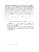
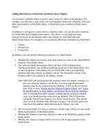
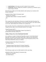
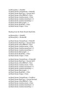


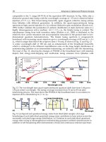
![[HeadWay] Phrasal Verbs and Idioms - Oxford University phần 2 pptx](https://media.store123doc.com/images/document/2014_07/13/medium_pks1405243208.jpg)