PARTICLE-LADEN FLOW - ERCOFTAC SERIES Phần 2 docx
Bạn đang xem bản rút gọn của tài liệu. Xem và tải ngay bản đầy đủ của tài liệu tại đây (1.01 MB, 41 trang )
Suspended sediment transport 33
∂u
∂t
+ u
∂u
∂x
+ w
∂w
∂z
= −g
∂ζ
∂x
+
∂
∂z
A
v
∂u
∂z
(2)
In these equations x, z represent the horizontal and vertical directions and u
and w the horizontal and vertical flow velocities. The variable t denotes time,
ζ is the water surface elevation, g is the constant of gravity and A
v
is the
constant eddy viscosity.
Boundary conditions at the bed disallow flow through the bottom (equation
3). Further, a partial slip condition compensates for the constant eddy vis-
cosity, which overestimates the eddy viscosity near the bed (equation 3). The
parameter S denotes the amount of slip, with S = 0 indicating perfect slip
and S = ∞ indicating no slip. At the water surface, there is no friction and
no flow through the surface (equations 4).
w −u
∂h
∂x
=0|
seabed
; A
v
∂u
∂z
= Su|
seabed
(3)
∂u
∂z
=0|
surface
; w =
∂ζ
∂t
+ u
∂ζ
∂x
|
surface
(4)
The flow and the sea bed are coupled through the continuity of sediment
(equation 5). Sediment is transported in two ways: as bed load transport (q
b
)
and as suspended load transport (q
s
), which are modeled separately. Here we
use a bed load formulation after [9] (equation 6).
∂h
∂t
= −
∂q
b
∂x
+
∂q
s
∂x
(5)
q
b
= α|τ
b
|
b
τ
b
|τ
b
|
− λ
∂h
∂x
(6)
Grain size and porosity are included in the proportionality constant α, τ
b
is
the shear stress at the bottom, h is the bottom elevation with respect to the
spatially mean depth H and the constant λ compensates for the effects of
slope on the sediment transport. For more details, we refer to [9] or [18].
In order to model suspended sediment transport q
s
, we describe sediment
concentration c throughout the water column, i.e. a 2DV model. Horizontal
diffusion is assumed to be negligible in comparison with the other horizontal
influences. The vertical flow velocity, w, is smaller than the fall velocity for
sediment, w
s
, and can be neglected in this equation, leading to equation (7).
This means that the sediment is suspended only by diffusion from the bed
boundary condition (equation 12). As the flow velocity profile is already cal-
culated throughout the vertical direction, suspended sediment transport q
s
can be calculated using equation (8).
∂c
∂t
+ u
∂c
∂x
= w
s
∂c
∂z
+
∂
∂z
s
∂c
∂z
(7)
34 Fenneke van der Meer, Suzanne J.M.H. Hulscher and Joris van den Berg
q
s
=
H
a
u(z)c(z)dz (8)
w
s
=
νD
3
∗
18D
50
(9)
D
∗
≡
g(s − 1)
ν
2
1/3
D
50
(10)
s
= A
v
(11)
The parameter
s
denotes the vertical diffusion coefficient (here taken equal
to A
v
), a is a reference level above the bed above which suspended sediment
occurs, D is the grain size. The dimensionless grain size is denoted by D
∗
,
(s − 1) is the relative density of sediment in water (
ρ
s
−ρ
w
ρ
w
), with ρ
w
the
density of water and ρ
s
the density of the sediment and ν is the kinematic
viscosity. Equations (9-11) are due to [18].
Suspended load is defined as sediment which has been entrained into the flow.
By definition, it can only occur above a certain level above the sea bed. At
this reference height, a reference concentration can be imposed as a boundary
condition. Various reference levels and concentrations exist for rivers, near-
shore and laboratory conditions. Those often applied are [17, 14, 5, 21]. For
offshore sand waves, the choice of a reference height is more difficult than it is
for the shallower (laboratory) test cases. In this case, the reference equation
of [17] (equation 12) is used, with a reference height of 1 percent of the water
depth, corresponding with the minimum reference height proposed in [17].
c
a
=0.015
D
0.01HD
0.3
∗
|τ|−τ
cr
τ
cr
1.5
(12)
The reference concentration at height a above the bed is given by c
a
and τ
cr
is the critical shear stress necessary to move sediment.
Both the gradient and the quantity of suspended sediment are largest close
to the reference height. Therefore, concentration values are calculated on a
grid with a quadratic point distribution on the vertical axis, such that more
points are located closer to the reference height and fewer points are present
higher in the water column. To complete the set of boundary conditions for
sediment concentration, we disallow flux through the water surface.
4Modelresults
In this paper, we concentrate fully on the influence of suspended sediment on
the initial state of sand waves. We started each simulation with a sinusoidal
bed-form with an amplitude of 0.1m.
Next, we investigated the (initial) growth rate and the fastest growing sand
wavelength (FGM). Table 1 shows some basic values used in the simulations
Suspended sediment transport 35
and the characteristics of the simulations are given in Table 2. Where possible,
typical values for sand waves in the North Sea are used. Note that ¯u is defined
as the depth-averaged maximum flow velocity.
Table 1. Parameter values for the reference simulation
parameter value unit parameter value unit
¯u 1m/s
v
0.03 m
2
/s
H 30 m
D 300 µm
A
v
0.03 m
2
/s w
s
0.025 m/s
S 0.01 m/s
a 0.3 m
α 0.3 -
Table 2. Simulations
simulation bed suspended varied simulation bed suspended varied
load load parameter
load load parameter
reference
√
3
√√
v
1
√√
- 4
√√
u
2
√√
ref. height a
5
√
-u
4.1 transport simulations
Figure 3(a) shows the growth rate for different sand waves lengths simulated
in the reference simulation. Moreover, the figure shows that the FGM is ap-
proximately 640m. For simulation 1, we included suspended sediment in the
reference computation. Figure 3(b) shows a comparison between the refer-
ence simulation and simulation 1. The growth rate is shown for a range of
wavelengths. Most remarkable is the increase of the growth rate by a factor
of approximately 10. This was unexpected as suspended sediment is assumed
to be of minor importance in these circumstances. The FGM for simulation 1
is 560m, 80m less than in the reference simulation.
In figure 4, the concentration profile in the water column at a crest point
over the tidal period is shown (upper figure), compared with the flow velocities
(lower figure). The sediment is only entrained into the first few meters of
the water column. The sediment concentration follows the flow without an
apparent lag, as the flow velocity near the bed is small and slowly changes over
time. However, these small variations in velocity are enough for the suspended
sediment to be entrained and to settle again within one tidal cycle. Close to
the reference height, the maximum sediment concentration is around 3·10
−4
m
3
/m
3
(0.8 kg/m
3
).
36 Fenneke van der Meer, Suzanne J.M.H. Hulscher and Joris van den Berg
200 300 400 500 600 700 800 900 1000
−3
−2.5
−2
−1.5
−1
−0.5
0
0.5
1
x 10
−8
wave length (m)
growth rate (1/s)
reference simulation
(a)
200 300 400 500 600 700 800 900 1000
−1
−0.5
0
0.5
1
1.5
x 10
−7
wave length (m)
growth rate (1/s)
reference simulation
simulation 1
(b)
Fig. 3. (a) Growth rate – reference simulation; (b) growth rate – simulation 1
(solid), compared with reference simulation (dashed). Parameters in Table 1.
Fig. 4. Sediment concentration (upper) and flow velocity (lower) on one location
over a tidal period, for simulation 1. More details see Fig 6 (upper).
4.2 sensitivity simulations
To study the influence of the reference height on the sediment entrainment
and suspended transport, the reference height in simulation 2 equation (12) is
200
300
400
500
600 700
800
900
1000
−1.5
−1
−0.5
0
0.5
1
1.5
x 10
−7
wave length (m)
growth rate (1/s)
simulation 1
ref heigth 1 cm
Fig. 5. Growth rate for simulation 2 (solid), compared to simulation 1 (dashed).
For simulation characteristics, see Table 1.
Suspended sediment transport 37
Fig. 6. Sediment concentration in the first 4 meters above a certain point of the
sand wave during one tide. Comparison between simulation 1 (upper) and 2 (lower)
decreased to 0.01m above the bed. This height is used as the lowest measurable
height for suspended sediment in shallow seas ([10, 6]). The results are shown
in figures 5 and 6. It can be seen in figure 5 that the growth rate decreases for a
lower reference height, whereas the FGM becomes 660m. Note that the growth
rate, compared to the situation without suspended sediment, is still larger. In
figure 6, it can be seen that, for the first 4 meters above the reference height,
no change occurs, except that the sediment is entrained about 0.30m higher
in the reference simulation. This difference is a direct result of the change
in reference height itself (from 0.30m to 0.01m). Therefore the difference in
growth rate is solely due to the contribution of these 0.29m to the integration
of u ·c over the water column.
Table 3. Simulation results, for varied values the first (second) value is for the
+50% (-50%) simulation
simulation FGM growth rate simulation FGM growth rate
(m) for FGM (1/s)
(m) for FGM (1/s)
reference 640 6.75e-9 3 860 - 350 1.24e-7 - 1.12e-7
1 560 1.29e-7
4 810 - 340 2.40e-7 - 3.87e-8
2 660 8.55e-8
5 670 - 610 1.23e-8 - 2.20e-9
In simulations 3 and 4, a sensitivity analysis was carried out for the diffusion
coefficient and the flow velocity. The value of sediment diffusivity,
v
,inthe
reference situation was assumed to be equal to the eddy viscosity Av, though
its value is not established. Both
v
and ¯u were varied by ± 50% of their
reference values. Their influence on the growth rate ω and the FGM are shown
in figures 7(a) and 7(b). It can be seen that the FGM increases significantly for
increasing
v
(FGM becomes 860m), and decreases for decreasing
v
(FGM
38 Fenneke van der Meer, Suzanne J.M.H. Hulscher and Joris van den Berg
200 300 400 500 600 700 800 900 1000
−2
−1.5
−1
−0.5
0
0.5
1
1.5
2
x 10
−7
wave length (m)
growth rate (1/s)
simulation 1
E
v
+50%
E
v
−50%
(a)
200 300 400 500 600 700 800 900 1000
−6
−5
−4
−3
−2
−1
0
1
2
3
x 10
−7
wave length (m)
growth rate (1/s)
simulation 1
u+50%
u−50%
(b)
Fig. 7. (a) Growth rate for simulation 3, variable
v
; simulation 1 (solid),
v
+50%
(dashed),
v
-50% (dotted). (b)Growth rate for simulation 4, variable ¯u; simulation
1 (solid), ¯u+50% (dashed), ¯u-50% (dotted).
300 400 500 600 700 800 900 1000
−1
−0.5
0
0.5
1
1.5
x 10
−8
wave length (m)
growth rate (1/s)
reference simulation
u+50%, no S
s
u−50%, no S
s
Fig. 8. Growth rate for simulation 5, variable ¯u and no q
s
; reference (solid), ¯u+50%
(dashed), ¯u-50% (dotted)
becomes 350m). The growth rate of the FGM remains of the same order
of magnitude. However, smaller wavelengths are damped more severely for
increasing sediment diffusivity.
For the flow velocity ¯u, the FGM again tends to increase with increasing ¯u
and vice-versa (for values, see Table 3), and smaller wavelengths are damped
moreforhighervaluesof¯u. For the growth rate, we now see a different effect.
As expected from the nonlinear ¯u in the sediment transport equation, the
growth rate is highly affected by ¯u. The higher the value of ¯u, the higher the
initial growth rate for the FGM.
As shown in figure 7(b), suspended sediment transport increases the effect
of variation in ¯u. If we compare this influence to the influence of varying ¯u
without suspended sediment transport (figure 8) it is clear that suspended
sediment increases the effect of changing velocities on the FGM (45% change
instead of 5% change in sand wavelength, for varying ¯u±50%). For the growth
rate of the FGM, this influence is less pronounced; the decrease (increase) of
Suspended sediment transport 39
growth rate with higher(lower) ¯u is 82% (67%) for the case without suspended
sediment and 86% (70%) for the case with suspended sediment.
5 Discussion and conclusions
In the reference simulation,
v
is assumed to be equal to the value of A
v
.
Various coupling equations exist to relate
v
to A
v
, varying from
v
being
larger than to being smaller than A
v
. [2] therefore assumed
v
equal to A
v
,
as no generally accepted method is available. Figure 7(a) shows that varying
the value of
v
influences the FGM significantly, though the growth rate itself
is hardly influenced. Possibly the large difference in growth rates between the
case with and without suspended load transport (reference simulation and
simulation 1) is caused, not by the value of
v
, but by the constant value of
both the eddy viscosity and sediment diffusivity. Due to these constant values,
A
v
might be overestimated near the bed, which is corrected for by the partial
slip boundary condition. Such a correction is not used for the
v
, possibly
leading to an increase of suspended sediment. Due to the constant
v
this
sediment can also be entrained higher into the water column.
Unfortunately, little field data for offshore sediment transport is available at
the moment, hindering a direct comparison with the results. [6] measured
suspended sediment offshore in the North Sea at a water depth of 13 meters.
Only during minor storms suspended sediment was detected. Maximal values
were around 2.3 kg/m
3
for 0.3m above the bed and 0.2 kg/m
3
for 1m above
the bed. For simulation 1, these values were 8 kg/m
3
and 0.34 kg/m
3
.[7]
measured sediment concentrations during a severe storm in the North Sea
close to the coast of the UK. They found, even under conditions of storm, finer
sediment (∼100µm) and a 25m water depth, that the sediment concentration
had decreased by about three orders of magnitude after 1 meter (± 40 kg/m
3
to 0.03 kg/m
3
). However, in the simulations this decrease was slower, leading
to higher concentrations higher in the water column (± 8 kg/m
3
close to
the reference height to 0.03 kg/m
3
at 3 meter above the bed). Although the
sediment concentration predicted in the model seems to be in a comparable
order of magnitude, transport rates are too large. The most likely cause is the
high entrainment of sediment into the water column. Further study on this
topic, and the effect of a depth dependent
v
is currently investigated.
As w turned out to be around an order of magnitude smaller then w
s
during
most of the tide, this term was neglected in the sediment continuity equation
(equation 7). However, for higher flow velocities or smaller grain sizes this
term will become more important. In that case w should be incorporated and
might increase the amount of suspended sediment during a part of the tidal
cycle on certain locations on the sand waves, leading to further growth or
decay of the sand waves. The effect depends on the specific locations (i.e.
crests or troughs) were suspended sediment will erode or deposit.
40 Fenneke van der Meer, Suzanne J.M.H. Hulscher and Joris van den Berg
[17] proposed a reference height for suspension with a minimum value of 1%
of the water depth. However, [19] stated that this leads to unrealistically high
reference levels in water depths of tens of meters. [19] therefore proposed to
use a reference height of 0.01m instead. [10] and [6] also used this height as the
lowest measurable height for suspended sediment in shallow seas. Both heights
are tested in simulations 1 and 2. They turn out to differ only in the lowest
part of the water column, which was excluded from the 1% (i.e. 0.3m) reference
height and included in the 0.01m alternative. Thus, the reference height does
not change the processes, but only includes or excludes the sediment in the
first view centimeters above the bed.
Based on grain sizes, [11] expected suspended transport for grains smaller than
230-300µm. Grains smaller than 170µm would be transported in suspension
only, in this case sand waves are rarely found. Recently, [20] showed that a
mixture of grain sizes leads to grain size sorting over sand waves, but hardly
affects the sand wave form and growth rate in the numerical code. Therefore,
in this paper we assumed grains of only one grain size, corresponding with
the medium grain size typically found on sand wave fields.
Concluding, the inclusion of suspended sediment transport in a sand wave
model demonstrates significant influences of suspended load on the initial
growth of sand waves. The influence of various parameters was investigated,
showing that the reference height for suspended sediment is of minor import-
ance, while the sediment diffusivity,
v
, and especially the depth averaged
maximum flow velocity, ¯u, largely influence both the FGM and the initial
growth rate. Further research will focus on fully developed sand waves and
the effects of wind and storm conditions, validated against field data.
Acknowledgment
This research is supported by the Technology Foundation STW, applied sci-
ence division of NWO and the technology program of the Ministry of Economic
Affairs. The authors are indebted to Jan Ribberink for his suggestions.
References
[1] Besio, G., Blondeaux, P., and Frisina, P. (2003). A note on tidally gen-
erated sand waves. J. Fluid Dynamics, 485, 171-190
[2] Blondeaux, P. and Vittori, G. (2005a). Flow and sediment transport
induced by tide propagation: 1 the flat bottom case. J. Geoph. Res. -
Oceans, 110 (C07020, doi:10.1029/2004JC002532)
[3] Blondeaux, P. and Vittori, G. (2005b). Flow and sediment transport
induces by tide propagation:2 the wavy bottom case. J. Geoph. Res. -
Oceans, 110 (C08003, doi:10.1029/2004JC002545)
[4] Buijsman,M. C. and Ridderinkhof, H. (2006). The relation between cur-
rents and seasonal sand wave variability as observed with ferry-mounted
adcp. In: PECS 2006, Astoria, OR-USA
Suspended sediment transport 41
[5] Garcia, M. and Parker, G. (1991). Entrainment of bed sediment into
suspension. J. Hydraulic Engg, 117 , 414-435
[6] Grasmeijer, B. T., Dolphin, T., Vincent, C., and Kleinhans, M. G.
(2005). Suspended sand concentrations and transports in tidal flow with
and without waves. In: Sandpit, Sand transport and morphology of off-
shore sand mining pits, Van Rijn, L. C., Soulsby, R. L., Hoekstra, P.,
and Davies, A. G.(eds.), U1-U13. Aqua Publications
[7] Green, M. O., Vincent, C. E., McCave, I. N., Dickson, R. R., Rees, J.
M., and Pearson, N. D. (1995). Storm sediment transport: observations
from the British North Sea shelf. Continental Shelf Res., 15 (8), 889- 912
[8] Hulscher, S. J. M. H. (1996). Tidal-induced large-scale regular bed form
patterns in a three-dimensional shallow water model. J. Geoph. Res.,
101, 727-744
[9] Komarova, N. L. and Hulscher, S. J. M. H. (2000). Linear instability
mechanisms for sand wave formation. J. Fluid Mech., 413, 219-246
[10] Lee, G. and Dade, W. B. (2004). Examination of reference concentration
under waves and currents on the inner shelf. J. Geoph. Res., 109 (C02021,
doi:10.1029/2002JC001707)
[11] McCave, I. N. (1971). Sand waves in the North Sea off the coast of
Holland. Marine Geology, 10 (3), 199-225
[12] Nemeth, A. A., Hulscher, S. J. M. H., and Van Damme, R. M. J. (2006).
Simulating offshore sand waves. Coastal Engineering, 53, 265-275
[13] Passchier, S. and Kleinhans, M. G. (2005). Observations of sand waves,
megaripples, and hummocks in the Dutch coastal area and their relation
to currents and combined flow conditions. J. Geoph. Res. - Earth Surface,
110 (F04S15, doi:10.1029/2004JF000215)
[14] Smith, J. D. and McLean, S. R. (1977). Spatially averaged flow over a
wavy surface. J. Geoph. Res., 12 , 1735-1746
[15] Van den Berg, J. and van Damme, D. (2006). Sand wave simulations
on large domains. In: River, Coastal and Estuarine Morphodynamics:
RCEM2005 , Parker and Garcia(eds.)
[16] Van der Veen, H. H., Hulscher, S. J. M. H., and Knaapen, M. A. F.
(2005). Grain size dependency in the occurence of sand waves. Ocean
Dynamics, (DOI 10.1007/s10236-005-0049-7)
[17] Van Rijn, L. C. (1984). Sediment transport, part ii: Suspended load
transport. J. Hydraulic Engineering, 11, 1613-1641
[18] Van Rijn, L. C. (1993). Principles of sediment transport in rivers, estu-
aries and coastal seas, vol. I11. Aqua Publications, Amsterdam
[19] Van Rijn, L. C. and Walstra, D. J. R. (2003). Modelling of sand transport
in DELFT3D-ONLINE. WL—Delft Hydraulics, Delft
[20] Wientjes, I. G. M. (2006). Grain size sorting over sand waves. CE&M
research report 2006R-004/WEM-005
[21] Zyserman, J. A. and Fredsoe, J. (1994). Data-analysis of bed concentra-
tion of suspended sediment. J. Hydraulic Engg, 120, 1021-1042.
Sediment transport by coherent structures in a
turbulent open channel flow experiment
W.A. Breugem and W.S.J. Uijttewaal
Delft University of Technology, Faculty of Civil Engineering and Geosciences,
Environmental Fluid Mechanics Section, P.O. Box 5048, 2600 GA Delft, The
Netherlands, ,
Summary. In order to obtain more insight into the vertical transport of suspended
sediment, an experiment was performed using a combination of PIV and PTV for
the measurement of the fluid and particle velocity respectively. In this experiment,
the particles were fed to the flow at 16 and 75 water depths from the measurement
section with an injector located at the centerline of the channel near the free surface.
At 16 water depths from the sediment injection, most sediment is still near the
free surface, and the sediment is transported downwards in sweeps, thus leading
to a mean particle velocity that is faster than the mean fluid velocity. It appears
that in this situation, downward going particles are indeed found in sweeps (Q4),
whereas upward going particles are preferentially concentrated in both Q1 and Q2
events. In the fully developed situation on the other hand, upward going particles
are preferentially concentrated in ejections, while downward going ones are found in
both Q3 and Q4 events, with a relatively increased frequency in Q3, and a decreased
one in Q4. The increased number of particles in Q2 and Q3, which have low fluid
velocities, leads to a mean particle velocity lower than the mean fluid velocity.
1 Introduction
The transport of suspended particles in turbulent flows is important in many
environmental flows. Therefore, much research already has been done. Never-
theless, modeling this highly complex phenomenon remains difficult.
The current state of the art in modeling sediment transport is by using
a two-fluid model [e.g. 18]. A vertical momentum balance for the dispersed
phase shows in the equilibrium situation (where the vertical accelerations and
gradients of the vertical particle velocity are negligible) the following relation
for the mean vertical particle velocity u
p,y
:
u
p,y
p
= u
f,y
f
+ u
f,y
p
+ u
y,T
(1)
Here, u
f,y
f
is the fluid velocity ensemble averaged over the fluid phase,
u
y,T
the still water terminal velocity, and u
f,y
p
, the drift velocity, i.e. the
Bernard J. Geurts et al. (eds), Particle Laden Flow: From Geophysical to Kolmogorov Scales, 43–55.
© 2007 Springer. Printed in the Netherlands.
44 W.A. Breugem and W.S.J. Uijttewaal
deviation of the mean fluid velocity as seen by the particles. The drift velo-
city results from averaging the relative velocity in the Stokes drag term of
this equation. Turbophoresis is neglected, because for almost neutrally buoy-
ant particles, it is counterbalanced by the pressure gradient working on the
particles. This agrees with our intuition that fluid particles in a fluid should
not concentrate near the wall. Equation 1 physically means that the mean
particle velocity (i.e. the flux per unit of concentration) is equal to the set-
tling velocity added to mean vertical fluid velocity and the extra drift term.
Simonin et al. [18] used a gradient diffusion hypothesis for the closure of this
term. In fact, the drift term is comparable to the c
v
term in conventional
advection-diffusion models.
The importance of the drift velocity in this modeling approach implies
that in order to understand dispersion, we need to know in which flow struc-
tures particles are located. It is already widely known that particles are not
necessarily distributed homogeneously in a turbulent flow. Preferential sweep-
ing [8], does not seem to be important for the situation we consider with a
relative density ratio ρ
p
/ρ
f
just above one, as the sweeping of particle out of
vortices by their inertia is compensated by the inward pressure gradient into
the vortex. Nevertheless, some DNS results show preferential concentration
for similar particles [19], but this seems to be mainly due to the initial condi-
tions [20]. Particles subjected to gravity but without inertia moving in cellular
flow fields were shown to have a complex behavior [12]. These particles can
either get trapped inside the vortex, leading to an upward drift velocity, or
remain outside the vortex, leading to a downward drift that enhances their
apparent settling velocity, but that does not change their slip velocity. The
combination of these two situations leads to a zero drift velocity for these
kind of particles in homogeneous isotropic turbulence. From the previous, it
appears that even particles without inertia can see a velocity field that is dif-
ferent from the overall velocity field, although not strictly due to preferential
concentration.
The objective of this study is to provide more insight in the behavior of
small, particles that are slightly heavier than the fluid and to find the flow
structures that cause the vertical transport of these particles. In order to
capture these flow structures, we perform an experiment, measuring simul-
taneously the fluid and particle velocities with Particle Image Velocimetry
(PIV) and Particle Tracking Velocimetry (PTV) respectively. We inject poly-
styrene particles near the free surface and perform measurements at either 16
or 75 water depths from the injection point. In the first situation, the highest
concentration is found near the free surface and the particles are on average
moving downwards, whereas in the latter situation, a fully developed situation
exists, in the wall normal direction. From now on, we will call the case with the
sediment inlet at 16 water depth from the measurement section the “settling
situation” and the one with the inlet at 75 water depths the “fully developed
situation”. The complete experimental setup is described in the next section.
In section 3, we show the mean profiles and probability density functions of
Sediment transport by coherent structures 45
the drift velocity and we compare them with the statistics at randomly gener-
ated particle locations. In section 4, we determine the conditionally averaged
drift velocity in the vicinity of a vortex head, followed by our conclusions in
section 5.
2 Experimental setup
Theexperimentswereperformedinanopenchannel,withalengthof23.5 m
awidthof0.495 m and a height of 0.50 m (fig. 1). The walls and bottom were
made of glass in order to have a hydraulically smooth boundary. In order to
perform the fluid velocity measurements using the PIV technique, the water
was seeded with 10 µm hollow glass spheres (ρ = 1100 kg/m
3
).
As pseudo-sediment, polystyrene particles with a mean diameter of 347 µm
were used, which had a density ρ
p
of 1035 kg/m
3
. The terminal velocity was
determined in still water as v
T
=2.2 mm/s, which compares well with the
expected value of 2.1 mm/s (Re
p
= v
T
d
p
/ν
f
=0.71).
Fig. 1. Experimental setup
The experiments were performed at Re =10, 000 (Re
∗
= 508), which
was obtained by setting the centerline velocity to 0.20 m/s and the water
depth h to 5.0 cm. This velocity was chosen to ensure a sufficient amount of
sediment was suspended (u
∗
/v
T
≈ 5). The particles were fed to the flow mixed
with water through a nozzle with an inner diameter of 1 cm at the channel’s
centerline and its center located at 0.7 cm below the free surface. The inflow
velocity was manually adjusted to the channel velocity. The position of the
nozzle was varied from 80 cm to 375 cm from the measurement section, i.e.
at x
in
/h =16andx
in
/h = 75. In the latter situations, the vertical particle
velocities were zero up to experimental accuracy, which means that a fully
developed situation exists. Apart from that, the statistics of that situation
46 W.A. Breugem and W.S.J. Uijttewaal
did not differ much from a preliminary test where the sediment was injected
at 160 water depths from the measurement section.
The volumetric sediment concentration that was introduced was 1.210
−2
.
For each set, a sequence of 15 × 300 double images was recorded at 2 Hz.It
was checked that the flow remained stationary for the time of the experiment.
For comparison, also four sets of 300 double images were recorded at a frame
rate of 2 Hz for the flow in the channel, without the nozzle and any sediment
input, which we will call the clear water flow (CWF) data.
A45mm x45mm measurement section was located at a distance of
14.25 m from the channel entrance. At this location, a combination of both
PIV and PTV was used to measure the streamwise and wall normal velocities
of the polystyrene particles and the ambient fluid.
The data were processed with a modified version of the method of Kiger
and Pan [9] to discriminate sediment from tracer particles. In this algorithm,
a median filter with a size of 7 pixels is applied to remove the image of the
tracer particles from the recorded images, resulting in an image of only the
sediment particles. A PTV algorithm [21], which uses the displacement of
the centroid of the particles to determine the particle velocities, was applied
to the image with only sediment particles. By subtracting the image of the
sediment particles from the original image, an image containing only the tracer
particles was obtained. A PIV algorithm [11] is applied to this tracer image
withfirsta64x64window(50%overlap)andthentwo32x32window
(75 % overlap) iterations. The results are postprosessed with a median filter
to eliminate vectors that differ significantly from their neighbours. This leads
to 126 x 126 vectors with distance of 0.37 mm (3.76 wall units) between
each other. The velocity vector nearest to the wall was at y+ > 30, where
the resolution is equal to approximately two Kolmogorov length scales. This
seems adequate for transport process as these are goverend mostly by the
large scale structure. Breugem and Uijttewaal [5] found that the fluid velocity
profiles measured with this resolution compared well to the law of the wall,
when using the friction velocity from a fit of the Reynolds stress profile. The
fluid Reynolds stress profile was found to be linear and the mean vertical fluid
velocity was found to be zero up to experimental uncertainty, which together
indicate that secondary currents are negligible as might be expected with the
present B/h ratio of 10.
3 One-point drift velocity statistics
The sediment concentration profile (fig. 2) shows a high concentration near
thefreesurfaceinthex
in
/h = 16 case, whereas it resembles the Rouse pro-
file with most sediment near the bottom in the x
in
/h =75case2.Inthe
same figure, the drift velocity profiles are also shown for both the settling
and the fully developed case. These are defined by performing a bicubic in-
terpolation of the PIV fluid velocities at the particle locations. It is clear that
Sediment transport by coherent structures 47
in the predominantly settling regime, the streamwise fluid velocity seen by
the particles is higher than the average streamwise fluid velocity, whereas the
opposite is true in the fully developed case. The latter result has been found
before by for example Kiger and Pan [10]. The wall normal drift velocity is at
first negative, meaning that the sediment particles see on average a downward
velocity, which brings them down even more rapidly than gravity does (as the
still water settling velocity is about 0.2u
∗
). In the fully developed situation,
the particles see on average an upward moving fluid velocity. From theory,
it is expected that the vertical drift is equal to the settling velocity, but in
the data, the drift is smaller (a maximum of 0.1u
∗
rather than the expected
0.2u
∗
). There are two reasons for this discrepancy. First of all, there is a bias in
the measured fluid velocity toward the particle velocity as a result of leftovers
of the particle images after median filtering the images, which decrease the
measured relative velocity. Furthermore, because the grid spacing of the PIV
has about the size of a particle diameter, the fluid velocity that is used for
determining the drift velocity by interpolation is not the undisturbed velo-
city, but rather the one that is affected by the disturbance field of the particle
itself. In case of a Stokes flow, which is not completely valid here as Re
p
of
a freely settling particle is 0.71, the velocity disturbance around a moving
particle needs about five particle diameters to decay [e.g. 4].
0 1 2 3 4
0
0.1
0.2
0.3
0.4
0.5
0.6
0.7
0.8
0.9
1
C / C
0
y/h
−0.8 −0.4 0 0.4
0
0.1
0.2
0.3
0.4
0.5
0.6
0.7
0.8
0.9
1
<u
f
>
p
−0.8 −0.4 0 0.4
0
0.1
0.2
0.3
0.4
0.5
0.6
0.7
0.8
0.9
1
<u
f
>
p
Fig. 2. Left: mean sediment concentration profiles. −◦−: x
in
/h = 16; −∗−:
x
in
/h = 75; Dashed line: Rouse profile. Middle: Drift velocity profile x
in
/h = 16;
Right: x
in
/h = 75; −✄ −: streamwise direction; −−: wall normal direction;
In order to determine which coherent structures are causing the drift velo-
city, we computed the probability density functions (pdf) at y/h =0.55 (fig.
3). From these figures, it is first of all clear that in both cases the particle
velocity and the drift velocity do not differ much. There is an asymmetry in
the data, showing stronger sweeps than ejections and showing significantly
less Q1 and Q3 events than Q2 and Q4. Yet, there exists a clear difference
between both cases, with the peak of the histogram in the settling case in the
Q4 quadrant, whereas it is at the center in the fully developed situation.
To determine in which flow structures, the particles are concentrated, we
first picked random locations in the measured flow fields using the same num-
48 W.A. Breugem and W.S.J. Uijttewaal
−4 −2 0 2 4
−3
−2
−1
0
1
2
3
u/u
*
v/u
*
−4 −2 0 2 4
−3
−2
−1
0
1
2
3
u/u
*
v/u
*
−4 −2 0 2 4
−3
−2
−1
0
1
2
3
u/u
*
v/u
*
−4 −2 0 2 4
−3
−2
−1
0
1
2
3
u/u
*
v/u
*
Fig. 3. PDF of particle velocity (left) and drift velocity (right) at y/h =0.55. The
settling case is shown above, the fully developed situation below. Each contour line
indicates a doubled probability density.
ber as the particles that were measured at this height. We computed the drift
velocity histogram for these random positions and subtracted this from the
one measured at the particle locations (fig. 4). This method was chosen, in
order to prevent the results from being biased by a different statistical con-
vergence or from interpolation effects, which would have been the case if we
would have simply subtracted the fluid velocity histograms. It appears that
in the settling case, the upward moving particles are found in all upward flow
structures (Q1 and Q2), whereas downward moving particles, which are much
more common than upward moving ones, are preferentially concentrated in
sweeps (Q4). This appears to happen over the complete water depth (not
shown), except near the free surface (y/h > 0.8) , where downward moving
particles are preferentially concentrated in both Q3 and Q4 events.
In the fully developed situation on the other hand, upward moving particles
are preferentially concentrated in ejections (Q2), whereas downward moving
particles are concentrated preferentially in inward interactions (Q3). Note
that, because Q4 events are much more common than Q3 events in an open
channel flow, particles end up about as many times in Q3 as in Q4 events
due to the preferential concentration (fig. 3). In this situation, the number of
upward and downward moving particles is equal at every flow depth except
near the bottom [see 5], just as was found by Kiger and Pan [10].
Sediment transport by coherent structures 49
−4 −2 0 2 4
−3
−2
−1
0
1
2
3
u/u
*
v/u
*
−4 −2 0 2 4
−3
−2
−1
0
1
2
3
u/u
*
v/u
*
−4 −2 0 2 4
−3
−2
−1
0
1
2
3
u/u
*
v/u
*
−4 −2 0 2 4
−3
−2
−1
0
1
2
3
u/u
*
v/u
*
−4 −2 0 2 4
−3
−2
−1
0
1
2
3
u/u
*
v/u
*
−4 −2 0 2 4
−3
−2
−1
0
1
2
3
u/u
*
v/u
*
Fig. 4. PDF of the increase of the PDF at y/h =0.55 with to respect to random
sampled particles for all particles (left), upgoing particles (middle), and downgoing
particles (right). The settling case is shown in the upper row, the fully developed
situation in the lower row. Each contour line indicates a doubled intensity and
negative values are indicated with dashed lines.
The results for the fully developed case agree with the data from Kiger
and Pan [10] at y/h =0.6(y+ = 340). Both the preferential concentration of
upgoing particles in ejections and of downgoing particles in inward interactions
(Q3) can clearly be seen in their data. A decreased number of particles in
sweeps and an increased one in ejections also agrees with the findings of Cellino
and Lemmin [6] and Nikora and Goring [14], who find larger than average
upward sediment fluxes (c
v
) in these quadrants, noting that an increased
upward flux in a sweep (i.e. in a downward flow structure) can only come
from a decreased concentration (because Cellino and Lemmin [6] do not find
the Reynolds stress contributions of the different quadrants to change with
respect to clear water flows). Cellino and Lemmin [6] do not find the increased
importance of Q3 events in their measurements. This may be attributed to the
larger concentration in their measurements, as Nikora and Goring [14] report
a large concentration dependence on the quadrant distribution with increased
contributions for Q1 and Q3 events and increased concentration fluctuations
in their low concentration cases.
50 W.A. Breugem and W.S.J. Uijttewaal
4 Spatial drift velocity structure
Here, we are interested in the conditionally averaged velocity field when there
is a vortex at a reference location x
0
. Conditional averaging is a widely used
tool in turbulence research. Unfortunately, statistical convergence is quite
slow, because only part of the data can be used to determine conditional
averages. A way to overcome this problem is the use of Linear Stochastic Es-
timation (LSE) [e.g. 1]. In LSE, a conditional average is approximated from
two-point correlations. In order to recognize the vortex, we use the fluctuating
part of the swirling strength λ
s
[22], which is scalar quantity.
The correlation functions were calculated for each PIV fluid velocity field
and then averaged over all 4500 realizations. Because of homogeneity in the
streamwise direction, the standard deviation and correlation function do not
change with x and therefore, only a reference height y
0
has to be chosen.
Because the LSE is linear in λ
s
, the exact value for this quantity is not im-
portant. It merely acts as a kind of threshold, and therefore a value of 1 /s
2
was used as was done before by Christensen and Adrian [7]. Swirling strength
does not detect the direction of the rotation, this in contrast to vorticity. Yet
it is known that both vortices in the direction of and opposite to the mean
shear are encountered in boundary layer turbulence [17]. Therefore, we cal-
culate the statistics conditioned on only those values of the swirling strength
for which ω
z
< 0, i.e. only for vortices that rotate with the mean shear.
The conditionally averaged fluid flow results for y
0
=0.5h are given in
figure 5. We use a streamline plot, rather than the normalized vector map
Christensen and Adrian [7] use to visualize the flow direction clearly even
at large distances from the hairpin vortex. In combination, we use a vector
plot without renormalization, which gives a clear impression of the size of the
structures. The swirling flow pattern is clearly visible at this location, and
it is also clear that a strong Q2 event can be found below the vortex head,
which extends over the complete water depth. This means that the whole
flow structure (vortex and the induced flow) can be classified as an attached
eddy. It is also interesting to note the absence of strong Q4 events in this flow
structure. A small Q3 event is visible upstream and below the vortex head.
The conditionally averaged drift velocity is shown in figure 6. Here, there is
a significant smaller number of vectors than in the fluid velocity LSE, because
larger bins were used in order to get converged statistics. Note that the drift
velocity, is not a zero-mean quantity (fig. 2). It appears that in the settling
case, the particles see large scale sweeps upstream and above the vortex head.
Around the vortex, it can be seen that the particles see an even intenser drift
at the downstream side of the vortex pulling the particles down around it.
In the fully developed case, the drift velocity again looks very similar to the
fluid velocity structure. Note that some care should be taken in interpreting
these results, because it does not show the amount of particles at a location
and some results therefore might be coming from a rather small number of
sediment particles and at the same time contribute little to the actual trans-
Sediment transport by coherent structures 51
port, as there are no particles at those locations. In the settling case, the
conditionally drift velocity becomes clearly smaller for a vortex higher in the
water column (not shown), with the most significant contribution above the
vortex head. In the fully developed situation on the other hand, the contri-
bution to the drift velocity becomes higher for vortices higher in the water
column (when its intensity is not changed), and it is located below the vortex
Fig. 5. Conditionally averaged fluid flow structure at y
0
=0.5h, calculated with
LSE. Only every other vector is shown.
−0.4 −0.2 0 0.2 0.4 0.6
0
0.2
0.4
0.6
0.8
1
r/h
y/h
−0.4 −0.2 0 0.2 0.4 0.6
0
0.2
0.4
0.6
0.8
1
r/h
y/h
Fig. 6. Conditionally averaged drift velocity structure at y
0
=0.5h.Leftforthe
settling case, right for the fully developed situation.
The clear difference between the conditional average of the drift velocity in
the settling case and the fluid velocity must mean that apparently only some
vortices are important for transporting the particles down in this case. I.e.,
although the downward and upward drifts are both related with a spanwise
vortex, the complete vortical structure transporting them is presumably very
52 W.A. Breugem and W.S.J. Uijttewaal
different. It appears that the concerned structure consists of a vortex head
with a sweep upstream and above of it. A model for this kind of structure
could be the type B eddies of Perry and Marusic [16], which consists of an
spanwise oscillating vortex tube, inclined 45 degrees in the streamwise dir-
ection and rotating with the mean shear. They proposed this structures in
order to obtain a better comparison with experimental data without claiming
their existence. Interestingly, a similar structure was found in conditionally
averaged structures by Adrian and Moin [2] in a DNS of a homogeneous shear
flow, related with Q4 events. Apparently, these second structures are much
less significant in a boundary layer than hairpin vortices, because in the con-
ditional average of the fluid velocity structure, no trace of them is visible. In
the fully developed situation on the other hand, it seems that hairpin vortices
are responsible for the drift velocity structure.
5Conclusion
We performed a PIV/PTV experiment in order to measure the drift velocity
statistics of pseudo sediment particles in a turbulent flow. We varied the dis-
tance between the introduction of sediment and the measurement location.
At 16 water depths from the measurement section, we found that most of the
sediment was still near the free surface and moving downwards, preferentially
concentrated in sweeps (Q4), whereas a smaller number of upward moving
particles are found both in Q1 and Q2 structures, thus causing the mean
particle velocity to be higher than the mean fluid velocity. A spatial view of
these structures shows that mainly the structures located above a spanwise
vortex head rotating with the shear, are important for this downward trans-
port. A possible eddy that could display this kind of behavior is the type B
eddy from Perry and Marusic [16]. The downward transport in this situation
seems to be quite similar to the increased apparent settling velocities in a
cellular flow field [12], where settling particles that are outside a vortex move
around that vortex at the down flowing side.
In the fully developed situation on the other hand, upward sediment trans-
port occurs in ejections, whereas downward transport occurs in inward inter-
action (Q3) and sweeps (Q4), although particles are found significantly more
in Q3 events than could be expected from random sampling, and significantly
less in Q4 events. The streamwise velocity that is lower than the mean in Q2
and Q3 events causes the mean streamwise particle velocity to be slower than
the mean fluid velocity. The ejections are clearly related to hairpin vortex
structures. In this situation, the number of upward and downward moving
particles is approximately equal.
The physical mechanism for the increased concentration in Q3 events in
the fully developed situation is shown in figure 7. Particles from the near
the bottom, where the largest concentration exists, are transport upwards
by an ejection related to a hairpin vortex. These hairpin vortices travel in
Sediment transport by coherent structures 53
Fig. 7. Physical mechanism of particle transport in the fully developed situation.
The image shows a hairpin vortex packet and two typical particles in a frame moving
with the hairpin vortex packet convective velocity. ISL: Internal shear layer, HPV:
Hairpin vortex
packets [3] and therefore a Q3 event related to an upstream hairpin vortex
can transport a part of the particles downwards (dotted in fig. 7). Another
part of the particles (filled in fig. 7) is transported upwards of the internal
shear layer that connects the two vortices. From there, it might remain at
the same vertical location [15], be transported further upwards by another
hairpin vortex packet or be transported down by a sweep (similar as what
happens in the settling case). Note that these light particles do not seem to
settle down by gravity [also found by 13], but are transported downwards by
coherent structures. Yet, the influence of gravity on the concentration profile
in the fully developed situation is evident.
Acknowledgment
This research is supported by the Dutch Technology Foundation STW, ap-
plied science division of NWO and the Technology program of the Ministry of
Economic affairs. The financial support from WL|Delft Hydraulics and KIWA
Water Research is highly appreciated.
References
[1] R.J. Adrian. Stochastic estimation of conditional structure: a review.
Applied Scientific Research, 53:291–303, 1994.
[2] R.J. Adrian and P. Moin. Stochastic estimation of organized turbulent
structure: homogeneous shear flow. Journal of Fluid Mechanics, 190:
531–559, 1988.
54 W.A. Breugem and W.S.J. Uijttewaal
[3] R.J. Adrian, C.D. Meinhart, and C.D. Tomkins. Vortex organization
in the outer region of the turbulent boundary layer. Journal of Fluid
Mechanics, 422:1–54, 2000.
[4] G.K. Batchelor. An introduction to fluid dynamics. Cambridge university
press, 1967.
[5] W.A. Breugem and W.S.J. Uijttewaal. A PIV/PTV experiment on sed-
iment transport in a horizontal open channel flow. In R.M.L. Ferreira,
E.C.L.T. Alves, J.G.A.B. Leal, and A.H. Cardoso, editors, River Flow,
volume 1, pages 789–798. Taylor & Francis, 2006.
[6] M. Cellino and U. Lemmin. Influence of coherent flow structures on the
dynamics of suspended sediment transport in open-channel flow. Journal
of Hydraulic Engineering, 130(11):1077–1088, 2004.
[7] K.T. Christensen and R.J. Adrian. Statistical evidence of hairpin vortex
packets in wall turbulence. Journal of Fluid Mechanics, 431:433–443,
2001.
[8] J.K. Eaton and J.R. Fessler. Preferential concentration of particles by
turbulence. International Journal of Multiphase Flow, 20(Suppl):169–
209, 1994.
[9] K.T. Kiger and C. Pan. Piv technique for the simultaneous measurement
of dilute two-phase flows. Journal of Fluids Engineering, 122:811–818,
2000.
[10] K.T. Kiger and C. Pan. Suspension and turbulence modification effects
of solid particulates on a horizontal turbulent channel flow. Journal of
Turbulence, 3(019):1–21, 2002.
[11] LaVision. FlowMaster Manual. PIV Hardware Manual for Davis 6.2.
Technical report, LaVision GmbH, February 2002.
[12] M.R. Maxey and S. Corrsin. Gravitational settling of aerosol particles
in randomly oriented cellular flow fields. Journal of the Atmospheric
Sciences, 43(11):1112–1134, 1986.
[13] B. Mutlu Sumer and R. Deigaard. Particle motions near the bottom in
turbulent flow in an open channel. part 2. Journal of Fluid Mechanics,
109:311–337, 1981.
[14] V.I. Nikora and D.G. Goring. Fluctuations of suspended sediment con-
centration and turbulent sediment fluxes in an open-channel flow. Journal
of Hydraulic Engineering, 128(2):214–224, 2002.
[15] Y. Ni˜no and M.H. Garc´ıa. Experiments on particle-turbulence interac-
tions in the near-wall region of an open channel flow: implications for
sediment transport. Journal of Fluid Mechanics, 326:285–319, 1996.
[16] A.E. Perry and I. Marusic. A wall-wake model for the turbulence struc-
ture of boundary layers. part 1. extension of the attached eddy hypo-
thesis. Journal of Fluid Mechanics, 298:361–388, 1995.
[17] L.M. Portela. Indentification and characterization of vortices in the tur-
bulent boundary layer. PhD thesis, Stanford University, 1997.
Sediment transport by coherent structures 55
[18] O. Simonin, E. Deutsch, and J.P. Minier. Eulerian prediction of the fluid
particle correlated motion in turbulent two-phase flows. Applied Scientific
Research, 51(1-2):275–283, 1993.
[19] K.D. Squires and H. Yamazaki. Preferential concentration of marine
particles in isotropic turbulence. Deep-Sea Research Part I, 42(11/12):
1989–2004, 1995.
[20] K.D. Squires and H. Yamazaki. Addendum to the paper ”preferential
concentration of marine particles in isotropic turbulence”. Deep-Sea Re-
search Part I, 43(11-12):1865–1866, 1996.
[21] G.A.J. van der Plas, M.L. Zoeteweij, R.J.M. Bastiaans, R.N. Kieft, and
C.C.M. Rindt. PIV, PTV and HPV User’s Guide 1.1. Eindhoven Uni-
versity of Technology, April 2003. Draft.
[22] J. Zhou, R.J. Adrian, S. Balachandar, and T.M. Kendall. Mechanisms for
generating coherent packets of hairpin vortices in channel flow. Journal
of Fluid Mechanics, 387:353–396, 1999.
Transport and mixing in the stratosphere: the
role of Lagrangian studies
Bernard Legras and Francesco d’Ovidio
Laboratoire de Meteorologie Dynamique, Ecole Normale Sup´erieure and CNRS, 24
rue Lhomond, 75231 Paris Cedex 05, France ,
www.lmd.ens.fr/legras
1 Introduction
The stratosphere is an important component of the climate system which
hosts 90% of the ozone protecting life from the ultra-violet radiations and,
through the region called upper troposphere / lower stratosphere (UTLS)
that encompasses the tropopause, has some control on the weather, the chem-
ical composition of the atmosphere and the radiative budget. Because the
temperature grows with altitude in the stratosphere, convection is inhibited
by stratification, and the motion is mainly layer-wise on isentropic surfaces,
with time scales of the order of weeks to months. The cross-isentropic adia-
batic circulation is slow with time scales of the order of the season to several
years. Below 30km, many chemical species, among which ozone, do not have
significant sources or sinks and exhibit a chemical life-time of the order of
several months to years. Such species can be treated as passive scalars trans-
ported by the flow. Their distribution is then dependent on the transport
and mixing properties. Two useful quantities are the potential temperature
θ = T (p
0
/p)
R/C
p
which is related to entropy by S = C
p
ln θ and the Ertel
potential vorticity (or PV) P =(∇×u·∇θ)/ρ which is a passive tracer under
adiabatic and inviscid approximation. Owing to the separation between fast
horizontal adiabatic motion and slow vertical diabatic motion, the potential
temperature is often used as a vertical coordinate. PV is not practically meas-
urable by in situ or remote instruments unlike many chemical tracers but can
be easily calculated from model’s output. It is most often used as a diagnostic
of transport and dynamical activity.
Observations by in situ instruments and remote sensing show that the
stratosphere exhibits well-mixed regions separated by transport or mixing
barriers. Particularly, in the winter hemisphere, two dominating barriers are
formed at the periphery of the polar vortex and in the sub-tropics that isolate
the mid-latitudes from both the polar and tropical regions [1]. Since vertical,
diabatically induced, motion is upward in the tropics and downward in the
extra tropics, with the largest descent within the polar vortex, vertical tracer
Bernard J. Geurts et al. (eds), Particle Laden Flow: From Geophysical to Kolmogorov Scales, 57–69.
© 2007 Springer. Printed in the Netherlands.
58 Bernard Legras and Francesco d’Ovidio
gradients are turned into step horizontal gradients on isentropes intersecting
the barriers. In the UTLS, the barrier associated with the subtropical jets
near 30N and 30S in latitude separates the upper troposphere from the lower-
most stratosphere on isentropic surfaces crossing the tropopause. The layer
of the stratosphere just above the tropopause undergoes exchanges with the
mid-latitude troposphere mainly due to upper level frontogenesis, which is a
consequence of baroclinic instability and/or intense convective events which
are often themselves associated with frontogenesis. At higher levels, that is
for 380K>θ>350K, the exchanges across the tropopause occur between
the lower stratosphere and the Tropical Tropopause Layer (TTL) which is an
intermediate region between the tropical convective layer and the stratosphere.
Figure 1 summarizes these processes.
Fig. 1. Scheme summarizing the Brewer-Dobson meridional circulation in the stra-
tosphere end exchange processes.
The scope of theory and modeling is to provide a qualitative and quantitat-
ive account of these observed properties. A number of progresses in this matter
over the last ten years have been due to the extensive usage of Lagrangian
calculations of parcel trajectories based on the analyzed winds provided by
the operational meteorological centers. It is the goal of this presentation to
review the ongoing work in this direction.
2 Isentropic stirring
The strong stratification of the stratosphere accompanied by weak net dia-
batic contribution constrains parcels to move on isentropic surfaces. Lag-
rangian isentropic motion differs from fully turbulent motion and is akin to
Transport and mixing in the stratosphere: the role of Lagrangian studies 59
two-dimensional turbulence or chaotic motion in a plane, where the flow is
smooth and advection is dominated by the large structures. Such dynamics is
known to produce transport barriers where tracer gradients intensify.
The effective diffusivity [2, 3, 4] has been used with success as a diagnostic
of such effects in atmospheric flows. The method applies to a tracer, usu-
ally PV, with a mean latitudinal gradient such that the longitude-latitude
coordinates can be replaced by the area of embedded tracer contours and an
azimuthal coordinate along the contours. By a weighted averaging along the
contours, the advection-diffusion equation ∂c/∂t + u∇c = κ∇
2
c is replaced
by a purely diffusive equation
∂C(A, t)
∂t
=
∂
∂A
κ
eff
(A, t)
∂C(A, t)
∂A
,
where A is the area of the contour γ(C, t) and the effective diffusivity is
κ
eff(A,t)
= κ
0
L
2
eq
(A, t)
A
4π −
A
r
2
(1)
with
L
eq
(A, t)=
γ(C,t)
|∇c|dl
γ(C,t)
1
|∇c|
dl ,
and r is the radius of the Earth. The device in (1) is to bind the complex
stirring of the passive scalar in the averaging over the contour. It can be shown
[5] that L
eq
is always larger than the actual length of the tracer contour but
that in practice the two quantities scale similarly. Hence, effective diffusivity is
small where the contours are less deformed, that is where transverse gradients
are less intensified, leading to less mixing.
Another measure of atmospheric stirring is provided by the local Lyapunov
exponent [6, 7] which estimates the Lagrangian stretching as the separation
rate of two close parcels over a given period of time or over a given growth.
Around the Antarctic stratospheric polar vortex, a minimum in both the
effective diffusivity and local Lyapunov exponent is observed along the streak
lines at the center of the jet [7, 8]. This minimum is surrounded by a very
active mixing region with large stretching where air is brought from and to
the mid-latitudes within a few days. However, the very stable Antarctic polar
vortex is rather an exception than the rule among atmospheric flows which
usually exhibit much less stable patterns. Over most of the atmosphere, the
Lyapunov exponents and effective diffusivity are rather anti-correlated than
correlated, contrary to the simple expectation.
The main reason of this discrepancy is that atmospheric flow, like most
quasi-2D flows, is dominated by extended shear regions that stretch material
lines but contribute weakly to the growth of tracer gradients. Let us first
consider the deformation of a small material circle surrounding a parcel at
time t. As time runs forward or backward, the flow defines a pair of linear