PARTICLE-LADEN FLOW - ERCOFTAC SERIES Phần 9 docx
Bạn đang xem bản rút gọn của tài liệu. Xem và tải ngay bản đầy đủ của tài liệu tại đây (642.24 KB, 41 trang )
338 M.G. Wells
Fig. 5. The laboratory experiment used to determine the influence of Coriolis forces
upon sedimentation patterns.
forms a weak turbidity current that is deflected to the right and is seen as the
black sediment at the base of the images.
The observed radius L of the sedimentation patterns are plotted in figure
7 and show an inverse dependence upon rotation rate f. In analogy to the
radius of the bulge of the buoyant river plume, we assume that the radius
of sedimentation on the rotating turbidity current is that which has Ro =1.
The Rossby number is defined as Ro = U/fL. The initial speed of collapse
of the turbidity currents is U ∼
√
g
h, so that the Rossby number is one
when L =
g
o
h/f. Based upon the low measured values of entrainment for
flows where Fr ∼ 1 in figure 4, we will assume there is little entrainment to
change the volume or g
. If we then use conservation of volume of the turbidity
current so that V = hL
2
π/4, the radius L of the quarter circle is related to
the reduced gravity, the initial volume and the Coriolis parameter by
L ∼ (4/π)
1/4
(g
o
V/f)
1/4
. (6)
This radius is similar to the scaling of non-sedimenting rotating experiments
by Hogg et al. (2001). In figure 7 there is good agreement between the scaling
(6) and the observed reduction in L with increasing f.
Influence of Coriolis forces on turbidity currents 339
Fig. 6. Eight images of the sedimentation patterns resulting from the release of
a black silicon carbide turbidity current in a rotating tank of area 1m
2
.Thetwo
dashed circles in each picture define the minimum and maximum estimates of the
radius L.
4 Applications to the 1929 Grand Banks earthquake
The 1929 earthquake off the Canadian coast of Nova Scotia triggered a tur-
bidity current which spread a 1.5 thick layer of sediment over 280,000 km
2
of
the sea floor (Piper et al. 1987). Heezen & Ewing (1952) calculated the speed
of the turbidity current based on the times that the trans-Atlantic telegraph
service was interrupted, and found that speeds varied from 25 m s
−1
on the
continental slope to under 4 m s
−1
on the flat abyssal plain. The time for
propagation of the current from the shelf to the deepest regions of the flat
abyssal plain 800 km away was about 12 hours, comparable to the inertial
period, T
in
=2π/f, of about 19 hours (Nof 1996). Thus the Earth
˜
Os rotation
should determine the radius that the turbidity current reaches and the res-
ulting sedimentation patterns. A simple estimate on the size of the turbidite
is then that Ro = 1 or that L ∼ U/f. If we use the speed estimates based on
Heezen & Ewing (1952), that U =25ms
−1
and that f =9.5 × 10
−5
s
−1
at
40
o
North then this implies that the radius of deposition is L = 250 km. In
figure 8 we see that this compares favorably with the distribution of sediment
observed by Piper et al. (1985).
5 Conclusions
The experiments described in this paper clearly show two strong effects of
rotation upon the dynamics of density or turbidity currents. Firstly rotation
340 M.G. Wells
(a)
(b)
Fig. 7. The experimentally determined radius of sedimentation in figure 6 is plotted
as a function of Coriolis frequency f , along with the theoretical predication that
L =1.06(g
V/f)
1/4
in a). The Rossby number for all the experiments can be seen
to be close to one in b) where we plot
√
g
V/L
2
f.
controls the entrainment ratio in such currents, as the velocity is in geo-
strophic balance. Our theoretical prediction that E ∼
√
g
/f
√
h showed good
agreement with experimental results in figure 4. Secondly we showed that the
radius of a large turbidity current influenced by Coriolis forces is comparable
the Rossby radius of deformation, so that the deposition patterns of turbidites
should be determined by (6) or L ∼ U/f. This theoretical prediction again
showed good agreement with laboratory experiments.
As there is an inverse dependence of speed and the deposition radius upon
the Coriolis parameter, these effects should be most striking for high latit-
Influence of Coriolis forces on turbidity currents 341
Fig. 8. a) The distribution of turbidites after the 1929 earthquake is shown in
grey on this contour map. Most of the sediment lies within 250 km of the canyon
mouth, but a small tongue of sediment between 0-50 cm thickness extends south for
approximately 600 km. Modified from Piper et al. (1985). b) A simplified conceptual
drawing of the sediment distribution, showing a quarter circle of radius 300 km from
the point where the turbidity current entered onto the abyssal plain, within this
radius lies all of the turbidite between 50-200 cm thickness.
ude turbidity currents and their resulting turbidites. We predict that at high
latitudes the turbidites would be of smaller spatial extent and have thicker
deposition patterns (assuming similar initial conditions). We found favorable
comparisons of the order of magnitude of the spatial extent of 1929 Grand
Banks turbidite with the Rossby number scaling. Future work will compare
these predictions with a more extensive set of geological observations at dif-
ferent latitudes.
References
[1] Alavian, V. (1986) Behavior of density currents on an incline. J. Hy-
draulic Eng. 112:27–42
[2] Cenedese, C., Whitehead, J.A., Ascarelli, T.A. & Ohiwa, M. (2004) A
dense current flowing down a sloping bottom in a rotating fluid. J. Phys.
Oceanog. 34:188–203
342 M.G. Wells
[3] Dallimore, C.J., Imberger J., & Ishikawa, T. (2001) Entrainment and tur-
bulence in saline underflow in Lake Ogawara. J. Hydraul. Eng. 127:937–
948
[4] Davies, P.A., Wahlin, A.K. & Guo, Y. (2006) Laboratory and analytical
model studies of the Faroe Bank Channel deep-water outflow. J. Phys.
Ocean. 36:1348-1364
[5] Ellison, T.H. & Turner, J.S. (1959) Turbulent entrainment in stratified
flows. J. Fluid Mech. 6:423–448
[6] Emms, P.W. (1999) On the ignition of geostrophically rotating turbidity
currents. Sedimentology 46:1049–1063
[7] Etling, D., Gelhardt, F., Schrader, U., Brennecke, F., Kuhn, G., Chabert
d’Hieres, G. & Didelle, H. (2000) Experiments with density currents on
a sloping bottom in a rotating fluid. Dyn. Atmos. Oceans. 31:139–164
[8] Griffiths, R.A. (1986) Gravity currents in rotating systems. Ann. Rev.
Fluid Mech. 18:59–89
[9] Hallworth, M.A., Huppert, H.E. & Ungarsish, M. (2001) Axisymmet-
ric gravity currents in a rotating system: experimental and numerical
investigations. J. Fluid Mech. 447:1–29
[10] Heezen, B.C. & Ewing, M. (1952) Turbidity currents and submarine
slumps, and the 1929 Grand Banks earthquake. Am. J. Sci. 12:849–873
[11] Hogg, A.J., Ungarish, M. & Huppert, H.E. (2001) Effects of particle sed-
imentation and rotation on axisymmetric gravity currents. Phys. Fluids
13:3687–3698
[12] Horner-Devine, A.R., Fong, D.A., Monismith, S.G. & Maxworthy, T.
(2006) Laboratory experiments simulating a coastal river inflow. J. Fluid
Mech. 555:203–232
[13] Huppert, H.E. (1998) Quantitative modelling of granular suspension
flows. Proc. Royal Soc. 356:2471-2496
[14] Jacobs, P. & Ivey, G.N. (1998) The influence of rotation on shelf con-
vection. J. Fluid Mech. 369:23–48
[15] Kneller, B. & Buckee, C. (2000) The structure and fluid mechanics of
turbidity currents: a review of some recent studies and their geological
implications. Sedimentology 47:62–94
[16] Middleton, G.V. (1993) Sediment deposition from turbidity currents.
Annu. Rev. Earth Planet. Sci. 21:89–114
[17] Nof, D. (1996) Rotational turbidity flows and the 1929 Grand Banks
earthquake. Deep Sea Res. 43:1143–1163
[18] Parker, G., Fukushima, Y. & Pantin, H.M. (1986) Self-accelerating tur-
bidity currents. J. Fluid Mech. 171:145–181
[19] Piper, D.J.W., Shor, A.N., Far’re, J.A., O’Connell, S. & Jacobi, R. (1985)
Sediment slides and turbidity currents on the Laurentian Fan; sidescan
sonar investigations near the epicentre of the 1929 Grand Banks earth-
quake. Geology 13:538–541
[20] Price, J.F. & Baringer, M.O. (1993) Outflows and deep water production
by marginal seas. Prog. Ocean. 33:161–200
Influence of Coriolis forces on turbidity currents 343
[21] Princevac, M., Fernando, H.J.H. & Whiteman, C.D. (2005) Turbulent
entrainment into natural gravity driven flows. J. Fluid. Mech. 533:259–
268
[22] Shapiro, G.I. & Zatsepin, A.G. (1997) Gravity current down a steeply
inclined slope in a rotating fluid. Ann. Geophysicae 15:366–374
[23] Turner, J.S. (1986) Turbulent entrainment–the developement of the en-
trainment assumption and its application to geophysical flows. J. Fluid.
Mech. 173:431–471
[24] Ungarish, M. & Huppert, H.E. (1999) Simple models of Coriolis-
influenced axisymmetric particle-driven gravity currents. Int. J. Multi.
Flow 25:715-737
[25] Wells, M.G. & Wettlaufer, J.S. (2005) Two-dimensional density currents
in a confined basin. Geophys. Astro. Fluid Dyn. 99:199–218
[26] Wells, M.G. & Wettlaufer, J.S. (2006) The long-term circulation driven
by density currents in a two-layer stratified basin. J. Fluid. Mech. (ac-
cepted)
A stochastic model for large eddy simulation of
a particle-laden turbulent flow
Christian Gobert, Katrin Motzet, Michael Manhart
Fachgebiet Hydromechanik, Technische Universit¨at M¨unchen, Arcisstr. 21,
D-80333 M¨unchen, Germany
Summary. This paper focuses on the prediction of particle distributions in a flow
field computed by large eddy simulation (LES). In an LES, small eddies are not
resolved. This gives rise to the question in which cases these eddies need to be re-
constructed (modeled) for tracing particles. Therefore the influence of eddies on the
particles in dependence on eddy and particle time-scales is discussed. For the case
where modeling is necessary, a stochastic model is presented. The model proposed
is a model in physical space and not in velocity space, i.e. not the velocities of the
unresolved eddies but the effects of these eddies on particle positions are reconstruc-
ted. The model is evaluated by an a priori analysis of particle dispersion in turbulent
channel flow.
1 Introduction
Particle laden flows in nature often reach Reynolds numbers for which dir-
ect numerical simulation (DNS) is not possible on nowadays computers. For
detailed numerical predictions of such flows, large eddy simulation (LES) is
considered to be an appropriate method. This paper focuses on the simulation
of a particle-laden flow by LES.
In a LES, not all length scales of the turbulent fluctuations are resolved.
This can be described formally by applying a spatial filter to the velocity field.
To solve the Navier-Stokes equations for the filtered velocity fields, a subgrid-
scale (SGS) model is required which accounts for the effect of the unresolved
scales on the resolved ones (SGS stresses). In the present work, this model
is referred to as fluid SGS model. In order to evaluate the performance of a
fluid SGS model, an a priori analysis can be conducted. In such an analysis,
the SGS-stresses are computed explicitly on the basis of an unfiltered solution
and its corresponding filtered one.
In many applications (e.g. prediction of sedimentation processes, disper-
sion of aerosols in the atmosphere) the dynamics of the carrier fluid is only
of secondary interest. It is more important to predict the distribution of the
suspended phase. Therefore only the scales in the carrier fluid which have a
Bernard J. Geurts et al. (eds), Particle Laden Flow: From Geophysical to Kolmogorov Scales, 345–358.
© 2007 Springer. Printed in the Netherlands.
346 Christian Gobert, Katrin Motzet, Michael Manhart
significant influence on the suspended phase must be computed. Nevertheless,
these scales are often too small to be resolved by LES; the corresponding ed-
dies might be in the subgrid range and a particle-SGS model will be required.
In the present work we focus on such cases. We compute the carrier fluid by
a LES and the suspended phase by solving the transport equation of particles
in a Lagrangian framework. Effects of the suspended phase on the carrier
flow as well as particle-particle interactions are neglected. For the effect of
the unresolved eddies of the carrier fluid on the particle motion, a stochastic
particle SGS model is developed. This model is validated by an a priori ana-
lysis conducted for dispersion in turbulent channel flow. The carrier fluid is
computed by DNS and subsequently filtered to eliminate errors that would
be introduced by a fluid SGS model.
It will be shown that the SGS eddies are most important for computing
particle distributions if the relaxation time of the particles is small. There-
fore we restrict the development and validation of the model on inertia free
particles.
This paper is organized as follows: In sections 2 and 3, the governing equa-
tions and numerical methods for DNS of the carrier flow and the suspended
phase are presented. In section 4, we discuss the significance of the subgrid
scale (SGS) velocities on the suspended phase. For the case where these velo-
cities are significant, we propose a stochastic model for including their effects
on the suspended phase. This model is developed in section 5 and verified by
an a priori analysis in section 6.
2 Numerical simulation of the carrier fluid
In order to conduct an a priori analysis, in this study a DNS of the carrier
fluid is performed by solving the Navier Stokes equations
div u =0 (1)
Du
Dt
= −
1
ρ
∇p + ν∆u. (2)
Here, u represents the fluid velocity, ρ the density, ν the kinematic viscosity
and p the pressure.
D
Dt
=
∂
∂t
+ u.∇ denotes the material derivative.
For solving equations (1) and (2), we used a Finite-Volume method. This
method is a modified version of the projection or fractional step method
proposed independently by [2, 20]. For spatial discretization a second order
scheme (mid point rule) was implemented. For advancing in time, we use a
third order Runge-Kutta scheme as proposed by Williamson [22] with constant
time step ∆t. The continuity equation (1) is satisfied by solving the Poisson
equation for the pressure. In this paper, we investigate turbulent channel flow
only. Therefore the Poisson equation can be solved by a direct method using
Fast-Fourier transformations in the homogeneous streamwise and spanwise
A stochastic model for LES of a particle-laden turbulent flow 347
directions of the channel flow and a tridiagonal solver in wall-normal direc-
tion. For a detailed description of the implemented flow solver the reader is
referred to [13]. Please note that in [13] a second-order scheme for advancing
in time was used whereas here, we implemented a third order Runge-Kutta
scheme.
We use periodic boundary conditions in the two homogeneous directions
and no slip conditions at the walls. The flow is driven by a constant pressure
gradient that adjusts the Reynolds number based on the half channel height
H and the bulk velocity u
bulk
to Re = 2817. This corresponds to a wall units
based Reynolds number of Re
τ
= 180. In our coordinate system, x is pointing
in streamwise, y in spanwise and z in wall-normal direction. The size of our
computational domain is 9.6H in streamwise, 6.0H in spanwise and 2.0H in
wall normal direction. For all computations staggered Cartesian grids were
used.
FortheDNSweused96×80×64 grid cells. The cell distance in wall units in
streamwise and spanwise direction is ∆x
+
=18and∆y
+
=13.5, respectively.
In wall normal direction a stretched grid was used with a stretching factor less
than 5%. Here, the cell width is ∆z
+
=2.7atthewalland∆z
+
=9.8atthe
channel center-plane. We compared our results up to second order statistics
with the spectral DNS of [8] and found excellent agreement. Further valida-
tions of the solver are given in [12, 13]. For evaluating the grid dependency on
the suspended phase, further computations were conducted on a refined grid.
This grid was obtained by refining the grid mentioned above by a factor of 2
in each direction, i.e. the number of grid cells was incremented by a factor of
8.
For the a priori analysis, the fluid velocity was filtered by top-hat filters
using a trapezoidal rule. Most of the results presented in this study are based
on a three dimensional filter with a filter width of 4 cell widths in each direc-
tion. This filter will be referred to as fil3d. Please note that this filter does
not correspond to filtering over a cube due to the different cell widths in each
direction. For analyzing anisotropic effects we implemented a two dimensional
top-hat filter which filters in spanwise and wall normal direction only (fil2d).
In these directions again the filter width was chosen to be 4 cell widths. For a
detailed investigation on the effect of different filters in a particle laden flow,
the reader is referred to [1].
3 Numerical simulation of the suspended phase in a DNS
For computing the suspended phase, single particles are traced. In all compu-
tations, only effects of the fluid on the particles are considered; effects of the
particles on the fluid are neglected (one way coupling). For computing traces
of particles other than fluid particles it is assumed that the acting forces on
these particles are given by the Stokes drag, fluid acceleration force and grav-
ity. Hence, according to Maxey and Riley [14] the equation of motion for a
348 Christian Gobert, Katrin Motzet, Michael Manhart
particle is given by
dv
dt
= −
c
D
Re
P
24t
P
(v − u)
Stokes drag
+
ρ
ρ
P
Du
Dt
fluid acceleration
+
ρ
P
− ρ
ρ
P
g
gravity
. (3)
Here, v(t) denotes the particle velocity, ρ
P
the density of the suspended phase
and g the gravity. t
P
is the particle relaxation time, i.e. the timescale for
the particle to adopt to the velocity of the surrounding fluid. The particle
Reynolds number Re
P
is based on particle diameter and particle slip velo-
city u − v which leads to a nonlinear term for the Stokes drag. The drag
coefficient c
D
was computed in dependence of Re
P
according to the scheme
proposed by Clift et al. [3].
Du
Dt
as well as the fluid velocity u must be evalu-
ated at the particle position x
P
(t), i.e.
Du
Dt
=
Du
Dt
(x
P
(t),t)andu = u(x
P
(t),t).
Hence, these values must be interpolated (see below).
In the cases which we considered in this study (for parameters cf. section
4), we found the Stokes drag to be a stiff term whereas fluid acceleration
force as well as gravitation are independent of v and thus not stiff. There-
fore it is appropriate to solve equation (3) by a numerical scheme that can
treat stiff terms and non stiff terms separately. Such a scheme is given by a
Rosenbrock/Wanner method [7]. Here, in each time step the stiff term (i.e. the
Stokes drag) is linearized and discretized by an implicit Runge-Kutta scheme.
For the other terms an explicit Runge-Kutta method is used.
The stiffness is dependent on particle properties. In order to trace different
suspended phases, an adaptive method was chosen. Altogether we decided to
implement the adaptive Rosenbrock/Wanner scheme of 4th order together
with an error estimation of 3rd order. This scheme can be found in [7].
In the remaining part of this section we will describe how we approximated
Du
Dt
(x
P
(t),t)andu(x
P
(t),t).
Let t
1
and t
1
+∆t be two instants at which the fluid velocity u is computed
on the given grid by solving the Navier-Stokes equations (1) and (2).
Du
Dt
equals the right hand side of the momentum equation (2) and is therefore also
computed on this grid at the given instants. Let t be some instant in between
two time steps of the flow solver, t
1
<t<t
1
+ ∆t. For computing the particle
velocity according to equation (3), the terms u(x
P
(t),t)and
Du
Dt
(x
P
(t),t)are
required. These can be obtained by interpolation in space (at x
P
)andintime
(at t).
The spatial interpolation uses a second order interpolation in direction of
the velocity vector and first order interpolation in the remaining directions.
This ensures a conservative interpolation which we found to be important for
the particle distributions. A change to a second order interpolation did not
affect the results significantly.
In detail, first u(x
P
(t
1
),t
1
)and
Du
Dt
(x
P
(t
1
),t
1
) were computed by spatial
interpolation. For the fluid acceleration force this was sufficient,
A stochastic model for LES of a particle-laden turbulent flow 349
Du
Dt
(x
P
(t),t) ≈
Du
Dt
(x
P
(t
1
),t
1
) ∀t
1
<t<t
1
+ ∆t. (4)
If this was done for u(x
P
(t),t) as well, this would correspond to a non-
continuous fluid velocity along a particle path. Due to the stiffness (v → u)
this would result in large amplitude higher order terms for v. An adaptive
solver would considerably reduce the time step size in such a situation which
would render the scheme ineffective. In order to circumvent this problem, we
approximated u during one time step ∆t linearly in time by using the flow
field of the previous time step t
1
− ∆t.
4 Influence of SGS velocities on the particles
In a LES context, not u but the filtered velocity
¯
u is computed. The question
at hand is whether replacing the velocity u by
¯
u in equation (3) has a signi-
ficant effect on the particle dynamics, i.e. if the non resolved eddies could be
neglected or not. This question will be addressed in the present section.
Consider a particle with a relaxation time t
P
residing in an eddy with a
much larger lifetime t
EL
, t
EL
t
P
. Here, it can be assumed that the particle
will eventually adopt to the eddy velocity. On the other hand, if the particle
relaxation time is large with respect to the eddy lifetime, t
EL
t
P
,the
eddy will disappear before the particle can adopt its velocity. Seen on the
timescale of the particle, this particle is pushed very slightly by such eddies.
Soon (referring to the timescale of the particle), the particle will be located
in the next eddy with t
EL
t
P
and the particle will be pushed again. For
such a particle, this will result in an effect similar to Brownian motion and
can therefore be considered as noise for the particles.
Concluding, the effect of a specific eddy on a particle is dependent on
t
EL
/t
P
. This was also found experimentally by Fessler et al. [5]. They invest-
igated the distribution of Lycopodium, glass and copper in air and found a
preferential concentration for Lycopodium but not for copper particles. This
is due to the different Stokes numbers St = t
P
/t
K
, t
K
being the Kolmogorov
timescale. For Lycopodium the Stokes number is St =0.6 whereas for copper
the Stokes number is St = 56.
As shown by Rouson and Eaton [18], the effect under consideration can be
shown by DNS at a lower Reynolds number at fixed Stokes number. We did
the same computations and found the results depicted in figures 1 and 2. The
flow field was computed as described above, i.e. at Re
τ
= 180, discretized on
96 × 80 × 64 cells. Recalling that the flow field in the two figures is identical
due to one-way coupling, it can be seen that the influence of an eddy varies
with the material properties of the particles.
For these computations we took Stokes drag, fluid acceleration and grav-
ity into account. The corresponding parameters were chosen in accordance to
the experiment by Fessler et al. Thus, Stokes numbers were chosen as stated
above for Lycopodium and copper resp., density ratio was ρ/ρ
P
=0.0017
350 Christian Gobert, Katrin Motzet, Michael Manhart
for Lycopodium and ρ/ρ
P
=0.000136 for copper. Gravity points in stream-
wise direction. For scaling gravity with the smallest eddies, particle Froude
numbers based on Kolmogorov scales Fr
P
=
√
ρ
P
η/
(ρ − ρ
P
)gt
2
K
were held
constant. Here, η is the Kolmogorov length scale. Thus, Fr
P
=1.9151 for
Lycopodium and Fr
P
=1.9136 for copper.
In contrast to our computations, Rouson and Eaton neglected fluid accel-
eration and gravity. We found good agreement between their results and ours.
Thus, in this case only Stokes drag affects the particle distribution signific-
antly. Hence, the influence of the eddies varies with the particle relaxation
time, the only material inherent parameter appearing in the Stokes drag.
Fig. 1. Lycopodium in air, instant-
aneous distribution on channel center-
plane, Re
τ
= 180, St =0.6
Fig. 2. Copper particles in air, in-
stantaneous distribution on channel
center-plane, Re
τ
= 180, St =56
In a LES, the size of the resolved eddies depends on the coarseness of the
LES grid. Equivalently, the minimal lifetime of the resolved eddies depends on
the LES cutoff frequency 1/t
LES
. According to this analysis, the SGS terms
are not negligible for tracing particles if t
LES
t
P
.Insuchacase,amodel
is required for recovering these effects. Evidently modeling is most important
if t
P
= 0, i.e. for tracer particles. Therefore a model can be evaluated by
applying it on such particles.
5 A stochastic SGS model
For cases in which SGS velocities cannot be neglected, several models were
already proposed by different authors. Some of these models are stochastic
[15, 19, 21], some are deterministic models [10, 15, 16].
In all the approaches mentioned, modeling is done in velocity space, i.e.
the SGS fluctuations u
are approximated. When modeling u
as a stochastic
variable, time correlations along the particle path must be included. Therefore
A stochastic model for LES of a particle-laden turbulent flow 351
in many of the models mentioned above, an additional differential equation
has to be solved.
In what follows, a SGS model for dispersion of inertia-free particles is
derived. Here, we propose to model the SGS-effect in physical space rather
than in velocity space. This will be explained as follows. For tracer particles
the particle position is given by
x(t)=x(0) +
t
0
¯u(τ)dτ
=:
¯
x(t)
+
t
0
u
(τ)dτ
=: x
t
. (5)
Here, ¯u(τ)=¯u(x(τ),τ)andu
(τ)=u
(x(τ),τ) are the filtered and SGS
velocities on a particle path, resp.
The filtered (i.e. resolved) velocities would result in deterministic particle
positions
¯
x(t). In our model, the non-resolved (SGS) velocities are considered
as random displacements, denoted here by x
t
. Thus, we propose to model x
t
as a stochastic process. To this end, we consider the moments of x
t
.Herewe
start with the model proposed by Shotorban and Mashayek [19]. This is a
model for the velocity fluctuations u
. Under the assumption of isotropic SGS
fluctuations they propose to solve for the SGS fluctuations at each time step
in a Lagrangian sense a stochastic differential equation
d¯u + du
= du =
−
1
ρ
∇¯p + ν∆¯u −
u − ¯u
T
L
dt +
C
0
sgs
dW
t
. (6)
Here, W
t
is a three dimensional Wiener process,
sgs
is the SGS dissipation
rate, T
L
is the lifetime of a representative SGS eddy and C
0
is a model con-
stant.
According to Deardorff [4],
sgs
can be computed by
sgs
=
ν
3
t
C
4
S
∆
4
(7)
with the Smagorinsky constant C
S
,filterwidth∆ and the eddy viscosity ν
t
.
In most LES models, the eddy viscosity is estimated from the gradients of the
resolved velocity field.
Combining the results of Gicquel et al. [6] and Lilly [11], a formula for the
SGS relaxation time T
L
can be obtained,
T
L
=
1
2
+
3
4
C
0
−1
∆
2
C
T
ν
t
(8)
352 Christian Gobert, Katrin Motzet, Michael Manhart
with another model constant C
T
which was set to 0.094 according to [6] and
[11].
Now we read the model by Shotorban and Mashayek in a LES context.
Therefore the filtered velocity in a Lagrangian framework can be written as
d¯u =
−
1
ρ
∇¯p + ν∆¯u − div τ
dt (9)
with τ being the SGS stress tensor. By subtracting equation (9) from equation
(6) a stochastic differential equation for the SGS fluctuations is obtained,
du
=
div τ −
u
T
L
dt +
C
0
sgs
dW
t
. (10)
Equation (10) is a linear stochastic differential equation. For such equa-
tions Kloeden and Platen [9] give differential equations for the first and second
moments of u
:
dE(u
)
dt
= −
1
T
L
E(u
)+divτ (11)
dE(u
2
)
dt
= −
2
T
L
E(u
2
)+2E(u
)divτ + C
0
sgs
(12)
Again, these equations are linear. Assuming a deterministic velocity for the
particles at t = 0, i.e. E(u
)(0) = E(u
2
)(0) = 0, the solution reads
E(u
)=T
L
(1 − e
−t/T
L
)divτ (13)
E(u
2
)=(T
L
div τ)
2
(1 + e
−2t/T
L
− 2e
−t/T
L
)
+
C
0
sgs
T
L
2
(1 − e
−2t/T
L
). (14)
Hence, the variance of the SGS fluctuations can be computed as
Var(u
)=E(u
2
) − E
2
(u
)=
C
0
sgs
T
L
2
(1 − e
−2t/T
L
). (15)
Equation (15) gives the variance for the SGS fluctuations in velocity space.
This information will be used now in order to compute the variance of the SGS
fluctuations in physical space, Var(x
t
). To this end, several assumptions will
be taken in the remaining part of this section. We will not present validations
for each assumption individually; instead, in section 6 results will be presented
which support the correctness of the resulting function Var(x
t
).
We start by integrating the model equation (10) under the assumption
that T
L
and
sgs
vary little
1
:
1
for a rigorous deduction the mean value theorem can be applied instead
A stochastic model for LES of a particle-laden turbulent flow 353
t
0
du
=
t
0
div τdt−
x
t
− x
0
T
L
+
C
0
sgs
W
t
(16)
Solving for x
t
gives
x
t
= x
0
+ T
L
⎛
⎝
−u
(t)+u
(0) +
t
0
div τdt +
C
0
sgs
W
t
⎞
⎠
. (17)
x
0
, u
(0) and
t
0
div τdt are deterministic. Thus,
Var(x
t
)=−Var (T
L
u
(t)) + Var
T
L
C
0
sgs
W
t
− 2T
2
L
C
0
sgs
Cov (W
t
, u
(t)) . (18)
Now we compute the covariance of the fluctuations and the Wiener pro-
cess generating the fluctuations, Cov (W
t
, u
(t)). For this we assume that the
fluctuation velocities are unbiased, E(u
(t)) = 0. Multiplication of (17) by
u
(t) and computing the expectation gives
t
0
E (u
(t)u
(s)) ds = −T
L
E(u
2
)+T
L
C
0
sgs
E (u
W
t
) (19)
Now we assume that the autocorrelation of the fluctuations decays expo-
nentially with the Lagrangian correlation timescale t
L
,
Cor(u
(t), u
(t + τ )) = e
−τ/t
L
. (20)
Furthermore in many applications one is interested in the long time behavior.
Therefore in the following we will consider large t only. According to equation
(14), E(u
2
) is constant for large t. Thus, by substituting (20) into (19) we
obtain
E(u
2
)(t
L
+ T
L
− t
L
e
−t/t
L
)=T
L
C
0
sgs
E (u
W
t
) . (21)
Substituting this into equation (18) gives
Var(x
t
)=C
0
sgs
T
2
L
(α + t
L
e
−t
t
L
)(1 − e
−2t
T
L
)+T
2
L
C
0
sgs
t (22)
α = −
3
2
T
L
− t
L
(23)
The first terms in equation (22) are exponentially decaying functions
whereas the last term is linear. This means that for large t the first terms
are negligible. We assume that these terms appear due to the suppression of
fluctuations at t =0,x
0
= u
(0) = 0. If the latter terms were random, the
exponential and constant terms in equation (22) might disappear.
Therefore we neglect these terms and model the SGS fluctuations accord-
ing to
354 Christian Gobert, Katrin Motzet, Michael Manhart
Var(x
t
)=T
2
L
C
0
sgs
t. (24)
One possibility to model x
t
with this variance is to model x
t
as a scaled Wiener
process. This is not only consistent with the derivation given but can also be
interpreted physically as dispersion. Armenio et al. [1] found that neglecting
SGS velocities results in a lack of dispersion. We want to compensate this by
modeling x
t
as scaled Wiener process:
dx
t
= T
L
C
0
sgs
dW
t
. (25)
This process can be implemented by adding in each time step of the flow
solver the appropriate stochastic term on the position of each particle:
x(t + ∆t)=x(t)+
t+∆t
t
¯
u dτ + T
L
C
0
sgs
∆t Z (26)
Z is a Gaussian distributed random variable with expectation 0 and variance
1. T
L
, C
0
and
sgs
can be obtained according to the model of Shotorban et
al. [19]. In our computations we implemented an explicit Euler scheme for
solving equation (26).
6 A priori analysis
In this section we present an a priori analysis of the SGS dispersion model
developed in section 5. For this analysis we distributed particles on the center-
plane of the channel described in section 2. Therefore each particle has the
same wall distance and by sampling over the particles, statistics in wall normal
direction can be obtained. All results will be displayed in wall units.
We traced the particles with velocities computed by DNS using the two
different grids described in section 2. During the simulations we stored the
particle positions on hard disk. In a post-processing step we computed the
variance of the wall normal coordinate of the particles which develops as
predicted by Pope [17] and computed by Armenio et al. [1] (cf. figure 3).
We compared both, coarse and fine grid simulations and decided that the
resolution of the coarse grid was sufficient for our purposes.
For conducting the a priori analysis, we filtered the DNS-velocity field by
top-hat filters as described in section 2. We traced particles with the filtered
velocities and found that the dispersion is reduced by filtering. This was
already found by Armenio et al. [1]. In contrast to their work, we filtered
also in wall normal direction. The corresponding variance of the particle po-
sition in wall normal direction (dispersion) is depicted in figure 3. Here, for
A stochastic model for LES of a particle-laden turbulent flow 355
both filters mentioned in section 2 the dispersion is depicted. Evidently dis-
persion in wall normal direction is not very sensitive to filtering in streamwise
direction.
In a LES context, we are interested in the SGS dispersion, i.e. the dif-
ference between dispersion computed by DNS and by filtered velocities. For
fil3d this SGS dispersion is plotted in figure 4. Please note that in such an
analysis the dependency of x
on ¯x is neglected whereas in our model this de-
pendency is respected due to adding the SGS dispersion subsequently during
the simulation. In order to validate the shape of the theoretically derived SGS
dispersion (equation (22)), we fitted the SGS dispersion according to equation
(22). The fit for t
L
=0.19,T
L
=0.001,C
0
sgs
T
2
L
= 1100 is also shown in fi-
gure 4. We find very good agreement between fitted function and numerically
computed SGS dispersion. This justifies the assumptions of section 5.
In the next step, we computed the particle positions with the filtered
velocities only and added subsequently the modeled SGS dispersion as given
by equation (26). For small time steps the stochastic term in equation (26)
(i.e. the contribution to the SGS dispersion) is so low that roundoff errors
become significant. In our simulations we used a time step for the flow solver
of ∆t =0.01
H
u
bulk
. We found that when using this time step in combination
with the filter fil3d these roundoff errors become dominant. In order to
compensate for this, we added the term corresponding to the SGS dispersion
at every 50 time steps only. The corresponding result is shown in figure 5.
It can be seen that for short times the deviation between DNS and modeled
result is still large whereas this becomes somewhat better for large times. This
was to be expected since we developed our model for long term behavior.
The difference occurs due to the neglecting of the constant and exponentially
decaying terms in equation (22). Therefore it is more appropriate to validate
the model on the dispersion rate, i.e. the time derivative of the dispersion.
This is plotted in figure 6. According to these results we are very satisfied
with the performance of our model.
356 Christian Gobert, Katrin Motzet, Michael Manhart
Fig. 3. Dispersion computed by DNS
and filtered velocities, displayed in
wall units.
Fig. 4. SGS dispersion and fit accord-
ing to equation (22).
Fig. 5. Dispersion computed by
DNS and filtered velocities as well as
filtered velocities plus modeled SGS
dispersion
Fig. 6. Rate of dispersion computed
by DNS and filtered velocities as
well as filtered velocities plus modeled
SGS dispersion
7 Conclusions
In this work we developed a stochastic SGS model for computing particle dis-
persion in turbulent flows. The model was developed for Eulerian-Lagrangian
simulations, i.e. where the fluid phase is computed by an Eulerian method and
the suspended phase is computed by tracing single particles in a Lagrangian
view. For such simulations the effect of the non resolved scales in the carrier
fluid must be modeled for tracing the suspended particles.
Modeling is done in physical space by subsequently adding a stochastic
term on the particle position which can be seen as dispersion caused by unre-
solved scales. For developing the model simplifications were taken which are
only valid when focusing on the long term behavior of the suspended particles;
the model is only capable of predicting the dispersion of particles when a cer-
A stochastic model for LES of a particle-laden turbulent flow 357
tain time after particle injection has passed. Since the model is of stochastic
nature, it can only be used for prediction of statistical properties.
In order to maximize the effect of subgrid scale influence, we focused on
tracer particles only in this study. An a priori analysis was conducted in
turbulent channel flow. Particles were released on the channel center-plane and
the evolution of particle dispersion was computed. In order to get a reference
solution, particles were traced by velocities computed from DNS. In another
simulation particles were traced by using filtered velocities and adding LES
dispersion as given by the model proposed. We found good agreement between
both simulations.
References
[1] V. Armenio, U. Piomelli, and V. Fiorotto. Effect of the subgrid scales
on particle motion. Physics of Fluids, 11(10):3030-3042, 1999
[2] A. J. Chorin. Numerical solution of the Navier Stokes equations. Math.
Comput., 22:745-762, 1968
[3] R. Clift, J. R. Grace, and M. E. Weber. Bubbles, Drops and Particles.
Academic Press, New York, 1978
[4] J. W. Deardorff. A numerical study of three-dimensional turbulent chan-
nel flow at large Reynolds numbers. J. Fluid Mech., 41:453-480, 1970
[5] J.R.Fessler,J.D.Kulick,andJ.K.Eaton.Preferentialconcentration
of heavy particles in a turbulent channel flow. Phys. Fluids, 6:3742-3749,
1994
[6] L. Y. M. Gicquel, P. Givi, F. A. Jabei, and S. B. Pope. Velocity filtered
density function for large eddy simulation of turbulent flows. Phys. Flu-
ids, 14:1196-1213, 2002
[7] E. Hairer and G. Wanner. Solving Ordinary Differential Equations II.
Stiff and Differential-Algebraic Problems. Springer Series in Computa-
tional Mathematics. Springer-Verlag, 1990
[8] J. Kim, P. Moin, and R. Moser. Turbulence statistics in fully developed
channel flow at low Reynolds number. J. Fluid Mech., 177:133-166, 1987
[9] P. E. Kloeden and E. Platen. Numerical solution of stochastic differen-
tial equations. Applications of mathematics. Springer Verlag, Berlin, 3
edition, 1999
[10] J. G. M. Kuerten. Subgrid modeling in particle-laden channel flow. Phys.
Fluids, 18:025108, 2006
[11] D. K. Lilly. The representation of small-scale turbulence in numerical
simulation experiments. In Proceedings of the IBM Scientific Computing
Symposium on Environmental Sciences, pages 195-210, 1967
[12] M. Manhart. Rheology of suspensions of rigid-rod like particles in tur-
bulent channel flow. Journal of Non-Newtonian Fluid Mechanics, 112(2-
3):269-293, 2003
358 Christian Gobert, Katrin Motzet, Michael Manhart
[13] M. Manhart. A zonal grid algorithm for DNS of turbulent boundary
layers. Computers and Fluids, 33(3):435-461, 2004
[14] M. R. Maxey and J. J. Riley. Equation of motion for a small rigid sphere
in a nonuniform flow. Phys. Fluids, 26:883-889, 1983
[15] N. A. Okong’o and J. Bellan. A priori subgrid analysis of temporal mix-
ing layers with evaporating droplets. Phys. Fluids, 12:1573-1591, 2000
[16] N. A. Okong’o and J. Bellan. Consistent large-eddy simulation of a tem-
poral mixing layer with evaporating drops. Part 1. Direct numerical sim-
ulation, formulation and a priori analysis. J. Fluid Mech., 499:1-47, 2004
[17] S. B. Pope. Lagrangian pdf methods for turbulent flows. Annu. Rev.
Fluid Mech., 26:23-63, 1994
[18] D. W. I. Rouson and J. K. Eaton. On the preferential concentration of
solid particles in turbulent channel flow. J. Fluid Mech., 428:149-169,
2001
[19] B. Shotorban and F. Mashayek. A stochastic model for particle motion
in large-eddy simulation. JoT, 7:N18, 2006
[20] R. Temam. On an approximate solution of the Navier Stokes equations
by the method of fractional steps (part 1). Arch. Ration. Mech. Anal,
32:135-153, 1969
[21] Q. Wang and K. D. Squires. Large eddy simulation of particle-laden
turbulent channel flow. Phys. Fluids, 8:1207-1223, 1996
[22] J. H. Williamson. Low-storage Runge-Kutta schemes. Journal of Com-
putational Physics, 35:48-56, 1980
Aggregate formation in 3D turbulent-like flows
A. Dom
´
inguez, M. van Aartrijk, L. Del Castello and H.J.H. Clercx
Fluid Dynamics Laboratory, Eindhoven University of Technology, Den Dolech 2,
5612 AZ, Eindhoven, The Netherlands.
Summary. Aggregate formation is an important process in industrial and environ-
mental turbulent flows. Two examples in the environmental area, where turbulent
aggregate formation takes place, are raindrop formation in clouds and Marine Snow
(aggregate) formation in the upper layer in the oceans.
The dispersion of inertial particles differs from that of (passive) fluid particles
and is dominated by particle-turbulence interaction. This is especially important
when the particle scales match the small-scale turbulent flow scales. Our motivation
to study turbulent aggregate formation comes from the need to describe aggregate
formation in small-scale turbulence in the oceans.
For a proper description, the study of aggregate formation in turbulent flows
requires a particle-based model, i.e. following single particles. Therefore, three main
processes should be modeled: the turbulent flow, the motion of the particles, and
the collision between particles and subsequent aggregate formation. In this study
we use 3D kinematic simulations to model the turbulent flow. A simplified version
of the Maxey-Riley equation is used to describe the motion of the particles. For
the collision and aggregate formation a geometrical collision check is used: when
the distance between two particles is smaller than the sum of their radii a collision
takes place. All the particles that collide stay together to form an aggregate, i.e.
100% coagulation efficiency. To account for the porosity of the aggregates a Fractal
Growth Model is used.
In this study the importance of the Stokes number and the fractal dimension
of the aggregates on collision rates and aggregate formation has been explored,
finding that the preferential concentration plays a very important role in aggregate
formation by creating regions of high particle concentration. Other results are: the
net effect of fractal growth is to increase the aggregate Stokes number and to decrease
the density of the aggregate.
In order to determine the performance and applicability of 3D-KS models on
aggregate formation processes, DNS simulations and supplementary laboratory ex-
periments are planned.
Bernard J. Geurts et al. (eds), Particle Laden Flow: From Geophysical to Kolmogorov Scales, 359–371.
© 2007 Springer. Printed in the Netherlands.
360 A. Dom
´
inguez, M. van Aartrijk, L. Del Castello and H.J.H. Clercx
1 Introduction
Phytoplankton populations in oceans are immersed in a turbulent environ-
ment. Turbulence increases encounter rates among plankton cells and other
organic and inorganic particles, promoting the formation of aggregates. These
aggregates are known as marine snow, and they are a vehicle for transporting
organic matter (CO
2
) to the bottom of the ocean [1]. The spectrum of spatial
and temporal scales in the ocean is extremely broad, ranging from kilomet-
ers to micrometers and from days to seconds. This makes direct numerical
simulation (DNS) of this system not feasible with the present computational
capacity. Implying that the large-scale modeling requires the use of empirical
models to be able to represent the effects of small-scale processes on large-
scale phenomena, i.e. to represent the gap between small- and large-scale phe-
nomena. Phytoplankton dispersion in large-scale simulations is an example.
In models the phytoplankton is usually represented as a passive tracer, but
under some conditions this representation fails. The transport of organic ma-
terial to the bottom of the ocean, also called the Carbon pump, is an example
of a process that cannot be described by considering plankton and particulate
matter as passive tracers. The net transport depends on the settling velocity
of individual particles which in turn depend in the particle-flow interaction.
The settling velocity of particles in turbulent flows is modified from the set-
tling velocity in quiescent fluids [2, 3] and particle properties can change by
particle-particle interaction (e.g. aggregation), or by particle-fluid interaction
(e.g. breaking up of aggregates). Therefore Lagrangian-based models follow-
ing trajectories of single particles are an ideal method to study aggregate
formation, where particle-particle and particle-flow interaction are import-
ant. These models capture in simplified ways these interactions, but they are
computationally expensive.
In general, when a few solid particles have formed an aggregate, the shape
of this aggregate is complex (although for many constituting particles the
aggregate can become more or less spherical). The aggregate is porous and its
density is different of that of the constituting particles. Aggregate growth is
known to be of fractal nature [4], and this fractal behavior should be taken in
account, although with a rather simplified model.
The inertial effects of plankton in turbulent flows have been studied pre-
viously by Squires and Yamazaki [5], finding that plankton can experience
preferential concentration. There are some works on aggregate formation:
turbulent aerosol aggregate formation using DNS [6]; polymer flocculation
in turbulent pipe flows [7] and aggregate formation in the ocean has been
explored with coagulation theory [8].
In the first part of this paper a brief theoretical introduction is presented.
The model is described in the second part, in the third section the results are
presented and conclusions are presented in the final section.
Aggregate formation in 3D turbulent-like flows 361
2 Turbulence-particle interaction
The interaction between a particle and a (turbulent) flow is complex. When
the volume fraction of the solid phase (particles), denoted by φ = NV
p
/V
d
(with N the total number of particles, V
p
the particle volume, and V
d
the
total volume of the system), is very small, say φ ≤ 10
−4
, the particles do
not influence the flow properties but the flow influences the particle traject-
ories. This is known as one-way coupling. Under different conditions particles
can act as passive tracers, showing a homogeneous distribution of particles
or, on the contrary, behave in ”resonance” with the flow, then showing pref-
erential concentration [9, 10]. This flow-particle interaction depends on the
combination of the particle and flow scales.
The smallest scales of the turbulent flow are the Kolmogorov time and
length scales,
τ
k
=
ν
ε
and η =
ν
3
ε
1/4
.
(1)
An important quantity characterizing the response of a particle of diameter
d
p
to the turbulent flow is known as the Stokes number and is given by
St =
τ
p
τ
k
(2)
where τ
p
, the particle response time. It is the time the particle needs to adapt
to a change in velocity and is given by
τ
p
= γ
d
2
p
18ν
(3)
where γ = ρ
p
/ρ
f
. This response time is valid for small spherical particles
with d
p
η. The particle-based Reynolds number Re
p
=
|u−v|d
p
ν
1, where
v is the particle velocity and u is the velocity of the fluid at the particle
position x.WhenSt 1 particles behave approximately as passive tracers
and they are homogeneously distributed in the flow domain. When St 1
particles respond to the smallest scales of the flow (τ
p
≈ τ
k
). The particles
are then ejected from the high-vorticity regions and accumulate in the high-
strain regions, thus giving rise to preferential concentration. Note that for
St 1 the particles are virtually insensitive to the small-scale turbulent
velocity fluctuations.
The equation of motion for a small, rigid spherical particle in the limit of
zero particle Reynolds number is given by the Maxey-Riley equation [11]
m
p
dv
dt
=6πaµ(u −v −
1
6
∇
2
u)+(m
p
− m
f
)g + m
f
Du
Dt
+
m
f
2
d
dt
(u − v −
1
10
∇
2
u)
+6πa
2
µ
t
0
d
dτ
(u − v −
1
6
∇
2
u)
dτ
πν
(t − τ)
,
(4)
362 A. Dom
´
inguez, M. van Aartrijk, L. Del Castello and H.J.H. Clercx
where a is the particle radius and µ is the dynamic viscosity of the fluid.
Furthermore, g is the gravitational acceleration, m
f
= ρ
f
V
p
and m
p
= ρ
p
V
p
,
with V
p
the particle volume, and ρ
f
and ρ
p
are the fluid and particle densities,
respectively. The forces appearing in the right hand side of (4) are: the Stokes
drag, the buoyancy force, the pressure gradient force, the added mass and
Basset history force, respectively. For particles with γ 1, often called heavy
particles, the only important forces are the Stokes drag and the buoyancy
force, and the resulting equation is:
m
p
dv
dt
=6πaµ(u − v)+(m
p
− m
f
)g. (5)
This study is restricted to turbulent dispersion and aggregation of heavy
particles.
3 Flow and aggregation model
The particle-based aggregation model described here consists of three parts:
the turbulent flow, the equation of motion for the particles and the collision-
aggregation process. The basic assumptions of the model are that at the smal-
lest scales of the flow the turbulence is homogeneous and isotropic, that d
p
η
and that φ<10
−4
to assume only one-way coupling and to consider particle-
pair collisions as the dominant process for aggregate formation.
3.1 3D Kinematic Simulations
Three-dimensional kinematic simulations (3D-KS) of turbulent flows [12] are
models of turbulent flows whose velocity field is constructed as a sum of ran-
dom Fourier modes with a prescribed Eulerian energy spectrum. The velocity
at position x and time t is given by:
u(x,t)=
N
k
n=1
[(A
n
×
ˆ
k
n
)cos(k
n
·x + ω
n
t)+(B
n
×
ˆ
k
n
)sin(k
n
·x + ω
n
t)], (6)
where N
k
is the number of modes in the simulation, A
n
×
ˆ
k
n
and B
n
×
ˆ
k
n
are spatial Fourier amplitudes,
ˆ
k
n
= k
n
/|k
n
| and k
n
is the wavenumber.
By construction, the velocity field satisfies the incompressibility condition
∇ · u = 0. The positive amplitudes of A
n
and B
n
are chosen according:
3
2
|A
n
| =
3
2
|B
n
| = E(k)∆k
n
, (7)
where E(k) is the Eulerian energy spectrum, ∆k
n
=(k
n+1
− k
n−1
)/2for
2 ≤ n ≤ N
k
− 1, ∆k
1
= k
2
− k
1
and ∆k
N
k
= k
N
k
− k
N
k
−1
. The distribution
ofwavenumbersisgeometric,
Aggregate formation in 3D turbulent-like flows 363
k
n
= k
1
L
η
n−1
N
k
−1
, (8)
where k
1
=2π/L and k
η
= k
N
k
=2π/η, the wave number associated with
the largest scale in the flow and the Kolmogorov length scale, respectively.
We are interested in modeling the so-called inertial range, where the energy
spectrum is given by:
E(k)=C
ε
ε
2/3
k
−5/3
k
1
<k<k
η
=0, otherwise
(9)
where ε is the energy dissipation rate, k is the wavenumber, C
ε
is an empirical
constant which value is chosen to be 1.5, according to Kraichnan [13]. The time
dependence of a turbulent flow is determined by the non-linear interaction
between different modes and by advection of the vorticity field by the velocity
field. However, in 3D-KS there is no dynamics and therefore the time evolution
of the flow is determined by the unsteadiness frequencies ω
n
in equation (6).
Following Fung [12], we choose the frequency of the mode n to be proportional
to the eddy turnover time associated with the wave-vector k
n
:
ω
n
= λ
k
3
n
E(k
n
), (10)
where λ is the unsteadiness parameter, and in this study λ =0.5. The resulting
velocity field incorporates turbulent-like flow structures, eddying, straining,
and streaming regions. Moreover, given the exact way in which the velocity
field is calculated we avoid interpolation errors calculating the velocities of
the flow at the particle position. One of the disadvantages of 3D-KS models
is the impossibility of having periodic boundary conditions.
3.2 Reduced equation of motion for the particle
The motion of the particles is calculated from equation (5) without the buoy-
ancy term, in order to understand as a first step solely the effects of inertia.
This assures that the collision rates are not affected by other processes like
differential sedimentation. So, the final equation used in this study is
m
p
dv
dt
=6πaµ(u − v). (11)
This equation is solved using a fourth order Adams-Bashforth (predictor)-
Adams-Moulton (corrector) method.
3.3 Collision-Aggregation
To explore aggregate formation we chose to start with a population of spher-
ical particles all having the same properties: all have diameter d
p
and density
![[HeadWay] Phrasal Verbs and Idioms - Oxford University phần 9 docx](https://media.store123doc.com/images/document/2014_07/13/medium_rpw1405243210.jpg)


![[Danh Nhân Việt Nam] Tiểu Sử Phan Đình Phùng phần 9 docx](https://media.store123doc.com/images/document/2014_07/14/medium_wpt1405279204.jpg)

