ATM BASICS - Chapter 2 pot
Bạn đang xem bản rút gọn của tài liệu. Xem và tải ngay bản đầy đủ của tài liệu tại đây (1.41 MB, 40 trang )
9
Chapter 2
How Does ATM Work
This chapter explains fundamental concepts that lay the basis for ATM
technology. The reader is given the in-depth understanding of the terms
such as ATM cells, statistical multiplexing, ATM switching and ATM layer
processing. The layers of ATM reference model are discussed and explained.
This in-depth view includes the Physical Layer, the ATM and the ATM
Adaptation Layer. The basic understanding of these terms is recommended
prior to reading through the following chapters.
2.1 ATM Protocol Reference Model
As it was mentioned before, ATM can be viewed as a part of the B-ISDN con-
cept. The development of B-ISDN protocols was facilitated by the definition
of the B-ISDN Protocol Reference Model (PRM). The model was developed
using the layered communication architecture based on the distinction
between layer functions developed by the ISO (International Standards
Organization). ATM plays a significant role in the B-ISDN PRM. The formal
ATM PRM is a three-dimensional model but the relations between layers
can be better viewed using one-dimensional layer model.
It is important to understand that the layers in the ATM PRM (presented in
the Fig.2-1) don’t have one-to-one mapping relationship with the seven lay-
ers OSI protocol reference model. Some of the layers of ATM PRM provide
the functionality of more than one OSI layer. For instance, the AAL (ATM
Adaptation Layer) represent some of the features of OSI layer 4 (transport
control), layer 5 (session control) and layer 7 (application control). Most of
the ATM PRM layers can be further subdivided into a number of sublayers.
2.2 Physical Layer
The physical layer (PHY) constitutes the lowest level of the ATM PRM. Its
major task is to transmit ATM cells between ATM devices over the physical
medium. ATM is designed to operate over potentially error free media.
Therefore, successful transmission of ATM cells between ATM devices
ATM Basics
10
Fig. 2-1, Simplified ATM Protocol Reference Model
requires very low values of BER (BER = 10
-12
or better). There exist today a
large variety of standards defining ATM physical interfaces. This situation
is mainly caused by a number of underlying technologies that can be used
by ATM.
2.2.1 Sub-layers
A physical layer takes complete cells from the mid-layer and transmits them
over the physical medium. The physical layer itself is subdivided into two
sub-layers:
•the Transmission Convergence (TC) sub-layer,
•the Physical Medium Dependent (PMD) sub-layer.
These two sub-layers work together to ensure that the physical interfaces
receive and transmit cells efficiently, with the appropriate timing structure
in place.
Chapter 2
11
Fig. 2-2, Sublayers of the Physical Layer
The Physical Medium Dependent is concerned with getting the bits on and
off the wire. The PMD bit transmission includes bit transfer and bit align-
ment. Technically, it covers bit timing, line coding, opto-electric conversion,
modulation and demodulation functions necessary to transfer bits over a
given medium. The physical connectors and signal characteristics differ
from medium to medium.
The Transmission Convergence sublayer is separated from details and char-
acteristics of the physical medium being used. Due to the presence of the
PMD sublayer the TC is specified independently of the underlying physical
medium and operates over different media. In general, the purpose of the
TC sublayer is to provide a uniform interface to the ATM layer in both direc-
tions. The cells received from the ATM layer are encoded and pushed into
the medium as a bit or a byte stream. The work of the TC sublayer can be
characterized by the following functions:
•Cell rate decoupling. This mechanism is used to insert idle cells in
the transmit direction in order to compensate for the variable rate of the
generation of ATM cells. At the receiving side all idle cells are identified and
suppressed.
•Header checksum generation and extraction. The TC sublayer can
detect and if necessary correct errors affecting the contents of the ATM cell
header. At the transmitting side the Header Error Check (HEC) field is gen-
erated in hardware and inserted into the cell header. At the receiving side
the HEC is recalculated and compared to the value that is extracted from
the header of the received cell. The capabilities of the algorithm used to cal-
culate the HEC allow for the detection and correction of single errors as well
as detection of double errors.
•Unpacking cells from the enclosing envelope. This function is also
referred to as cell delineation. The receiver must be able to recover the cell
boundaries. The TC sublayer must delineate the individual cells in the
received bit stream, either directly from the TDM frame or with the help of
the HEC field in ATM cells. This function can be complemented by the
scrambling/descrambling operation.
ATM Basics
12
•Frame generation. The cell flow must be adapted to the payload of
the transmission system in the transmit direction. In the receive direction,
the TC extracts the payload from the transmitted cell.
The separation between the TC and the PMD sublayers is the key factor
enabling flexibility in terms of variety of physical interfaces. Whereas the
PMD sublayer is different for different carriers and cables, the TC just sends
the cells as a string of bits to the PMD sublayer and converts the bit stream
into a cell stream for the ATM layer.
2.2.2 Physical Interfaces
ATM, while being an international transmission technology, has to be able
to work with a variety of formats, speeds, transmission media and distances
that may vary from operator to operator and from country to country.
Single-mode fiber, multi-mode fiber, coaxial pairs of different categories,
and shielded and unshielded twisted pairs are all standardized for the use
in the ATM environment. ATM can be also run over Radio Frequency
(RF)/satellite links. The ITU-T originally defined only two speeds, which
should be supported by ATM: 155.52 Mbps and 622.08 Mbps. However, over
time a number of additional speeds and interfaces have been defined, going
as low as DS1/E1 and as high as the 2.5 and 10 Gbps. The standardization
process of new physical interfaces is influenced by two factors. First of all,
new interfaces are standardized following the development of transmission
technologies (new types of o fibers and copper wires, e.g. UTP Cat. 6).
However in recent years a few standards have been introduced, while direct-
ly reflecting the market needs. Standards describing ATM over Fractional
Links, Inverse Multiplexing for ATM (IMA), Frame-based ATM Transport
over Ethernet (FATE) and Frame Based ATM over SONETS/SDH allow the
operators to maximize the efficiency of their network infrastructure.
Chapter 2
13
2.2 ATM Layer
The ATM layer deals with moving cells from a source to a destination, which
definitely implies the presence routing algorithms and protocols within the
ATM switches. From the functional point of view, the ATM layer performs
the work expected of the network layer in the OSI model. However, since
ATM is quite frequently used to transport IP packets, the ATM layer is by
many people characterized as a data link layer. This opinion is not precise
due to the fact that the ATM layer has also some characteristics of a net-
work layer: end-to-end virtual circuits, switching and routing. In result
ATM is sometimes referred to as a layer 2 ½ solution.
As it was mentioned earlier, the ATM layer is connection oriented, both in
terms of the services it can provide and the way it is used by the operators.
The basic concept present at the ATM layer is a virtual circuit (in official
ATM terminology called a virtual connection). A virtual circuit should been
seen as a connection from one source to one destination, although point-to-
multipoint connections are also supported. It is important to note that vir-
tual circuits are unidirectional but a pair of circuits is normally created at
the same time. The same identifiers are used for both directions of the vir-
tual circuit but the amount of reserved network resources can differ for both
directions.
The ATM layer is not guaranteed to be 100% reliable. The assumption has
been made that it’s the task of the underlying physical layer to ensure the
errorless transmission. Therefore, the ATM layer is unusual for a connec-
tion-oriented protocol in that it operates without any acknowledgements.
ATM Basics
14
2.2.1 ATM Cells
The ATM cell is probably the most obvious term for anyone who has ever
heard about ATM technology. The ATM cell, a very unique type of a packet,
is comprised of a 5-byte header and 48-byte payload that typically contains
user information. In total, ATM cells are 53-byte long (see in the Fig. 2-3).
The final agreement on the cell size was influenced by the struggle between
interests representing various interests. At the early stage of ATM stan-
dardization process in the ITU-T two different values of the payload size
were considered: 32-byte versus 64-byte value. The larger value was pro-
Chapter 2
15
Fig. 2.3, The ATM cell
posed by those who envisaged ATM as the technology satisfying data trans-
mission needs in the first place. In large cells the relation between the pay-
load and the total size is greater - the fixed size overhead represents the
smaller percentage of transmitted data. Hence, the overall efficiency for
data transmission is increased. The larger size of a cell, the greater amount
of the delay is experienced by other sources generating data in the form of
cells. This results in increased delays observed by real time applications
such as voice and video transmission. Needless to say, 32-octet payload
would be perfectly suited for the transmission of the E1 signal. The actual
decision on the 48-bytes payload size was a compromise trying to minimize
the disadvantages of two competitive proposals. It offered a tradeoff
between the efficiency for data transmission and the delay requirements for
data and video traffic. The size of ATM cells allowed operators to transmit
voice over relatively long distances (round trips of 1000 km) whilst avoiding
the need for expensive echo cancellers. The concept of fixed size cells is also
present in work done in Australia under development of DQDB (Distributed
Queue Dual Bus (DQDB), covered in IEEE 802.6. As the matter of fact, the
smallest unit of traffic in DQDB is the slot, which is of 53 bytes length.
2.2.2 ATM Cell Header
Fig. 2-4 shows the internal structure of an ATM cell header at UNI and
NNI. In ATM the interface between the user equipment and the ATM switch
is called User-to-Network Interface. All other interfaces, including those
between ATM switches and between ATM networks as referred to as Node-
to-Node Interfaces or Network-to-Node Interfaces. The key difference is the
Generic Flow Control (GFC) field, which is not present in cell headers trans-
mitted across the NNI.
ATM Basics
16
GFC (Generic Fow Control) is the 4-bit field that is present only in cells
transmitted between hosts and the network. Switches interfacing between
the user’s equipment and ATM network overwrite GFC, and it is not deliv-
ered to the destination. In early days of ATM it was intended to have some
utility for flow and priority control between hosts and the networks, when
multiple ATM devices were to be dropped on a single UNI. For any equip-
ment using uncontrolled access, the GFC files shouldn’t be used and the bits
must be always set to 0000 for the transmitted cells.
VPI (Virtual Path Identifier) has 8 bits available at the UNI and 12 bits
at the NNI, which gives either 256 or 4096 simultaneous virtual paths at
maximum per a physical connection.
Chapter 2
17
Fig. 2-4, The ATM cell header format
VCI (Virtual Channel Identifier) is the 16-bit field that selects a partic-
ular virtual channel within a given virtual path. It allows for up to 65,536
virtual channels per a virtual path. A number of combinations of VPI and
VCI values are reserved for control functions, such as setting up and clear-
ing virtual connections.
PTI (Payload Type Identifier) is the 3-bit field, which is as part of cell
control concept. The PTI defines the information carried in the cell payload.
User data and network management cells are differentiated due to the value
of the MSB bit (sometimes referred to as RM-celler). The second bit can be
used to indicate congestion affecting data traffic that can occur in the net-
work nodes. This bit is often called Explicit Forward Congestion Indicator
(EFCI). The LSB bit is used to indicate the final cell in the cell stream,
which has been filled with higher layer packet traffic. This bit is referred to
as the Service DataUnit (SDU) bit and its application is mostly related to
the presence of a certain adaptation layer type.
ATM Basics
18
Table 2-1, PTI field values
CLP (Cell Loss Priority) is the 1-bit field, which value is set by a host to
differentiate between high-priority and low-priority traffic. If the CLP is set
(CLP = 1) for a cell and the congestion occurs, the cell can be discarded at
switching devices. The cell can be directly marked as a low-priority cell by a
transmitting host or it can be tagged (CLP changes from 0 to 1) by an ATM
switch if the cell represents excessive traffic (breaking the traffic contract).
HEC (Header Error Check) is the 8-bit checksum field. The checksum
only covers the first four octets of the cell header. It is comprised of the
reminder of the 32 bits out of the header divided by the polynomial x
8
+ x
2
+
x + 1. Next it is added to the constant value of 01010101, which provides
robustness in the face of header that contain mostly 0 bits. The HEC scheme
can correct all single bit errors and detect multiple errors as well.
2.2.3 Cell Transmission
The first step in successful cell transmission is the computation of t the
header checksum. The decision to protect only the header was made delib-
erately to reduce the likelihood that some cells are delivered incorrectly due
to a header error. This operation does not involve any calculations over the
payload field and it’s up to higher layers to perform error detection and cor-
rection, if they desire so. This approach can be easily explained by taking
into account that most real-time applications, such as voice and video trans-
mission, accept occasional loss of information bits. However, this is not true
when it comes to data transmission.
Next, if the HEC has been generated and inserted into the cell header, it is
now possible to transmit the cell through the physical interface. Depending
on the type of transmission media, some additional operations may be nec-
essary. If an asynchronous medium is used, a cell can be sent without any
delay (no timing constraints are present). When a synchronous medium is
used, all cells must be sent according to a predefined timing pattern imposed
by the characteristics of a transmission medium. This may require the occa-
sional transmission of idle cells, which contain predefined and well-known
bit pattern.
Chapter 2
19
The ATM layer does not provide any mechanism that would allow for
acknowledgments. The actual reason is that the introduction of ATM coin-
cided in time with the envisaged rapid inclusion of high speed and very reli-
able fiber optic networks. It was thought that the task of efficient error con-
trol would be left to higher layers. And in fact, most transport layer proto-
cols handle this task sufficiently by re-sending the entire message if neces-
sary. ATM networks were intended for the use for real time traffic and for
that type of traffic re-transmitting a single
cell corrupted with errors is
more than problematic.
ATM cells belonging to a virtual connection are transmitted and delivered
to the destination in sequence. As can be easily noticed from the cell header
structure, there is no mechanism at the ATM layer that can provide a tool
for checking whether cells are delivered in sequence or not. Basically, it is
the matter of the transmission and switching concepts that ensures cell are
transmitted to the destination without reordering. Thanks to this assump-
tion large savings on cell processing delay are observed. However, the task
of checking the integrity of cell stream is given to higher layers of the ATM
protocol reference model.
2.2.4 OAM Cells
Within the stream of ATM cells carrying user data one it is possible to iden-
tify so called OAM (Operation And Maintenance) cells. These non-data ATM
cells are used by ATM switches for exchanging low level signaling and con-
trol information that are necessary for having the system running. The com-
mon application of OAM cells is to match the output ATM rate to the rate of
the underlying transmission technology. For instance, an ATM source trans-
mitting ATM cells over SONET would normally put out an OAM cell as
every 27 cells. In result, the data rate would slow the data rate down to
26/27 of 150,336 (OC-3) and thus match SONET completely.
ATM Basics
20
2.2.5 Cell Reception
At the receiving end an ATM device has to take incoming bits first, locate
the cell boundaries, check the header, processes the OAM cells (if there are
any) and finally pass the data cell up to the ATM layer. The most difficult
task is to delineate cell boundaries from the incoming bit stream. The delin-
eation algorithm has two forms that function in the same way. In non-
framed environment, the process is bit-aligned, while in a frame-based sys-
tem such as SONET, an octet-aligned process is a better solution. The gen-
eral rule is to obtain help from the HEC. The method is to initiate the delin-
eation process in a HUNT state (this is shown in Fig. 2-5) and to compute
the HEC value for any random sequence of 5 bytes (stored temporarily in a
40-bit shift register) and to consider these 5 bytes as a potentially valid cell
header. If this test fails, the next five bytes are taken into account. Given
the size of a header and an ATM cell, it can be derived that a header is going
to be located sooner or later. However, there may coincidently be a correct
calculation on what is not a header. In such a case the delineation procedure
will wait 48 bytes and try again. When the first calculation is completed suc-
cessfully, the process moves to PRESYNCH state, where again 48 bytes shift
takes place and repeated calculation is performed. If this wait-and-try-
process produces the correct answer δ times (typically 6 times), the delin-
eation process indicates SYNCH state. The value of δ is chosen to minimize
the probability of getting into SYNCH state by accident.
It may also happen that due to poor quality of transmission the synchro-
nization is lost. Some of the bits can be inserted or deleted from the trans-
mission. Then the cell with the bad header is discarded. But if α consecutive
HECs are bad, then the delineation process takes the decision that the syn-
chronization has been lost and it moves to the HUNT state.
Chapter 2
21
ATM Basics
22
The mechanism chosen for cell delineation requires that the TC sublayer is
able to understand and use the data included in the header of the ATM layer
present above it. This process in fact violates the basic rules of protocol engi-
neering as it requests that one layer makes the use of a higher layer.
Therefore, any change applied to the header format of the ATM layer would
affect the TC sublayer.
2.2.6 Virtual Channels and Virtual Paths
As it was stated earlier, the ATM layer provides connectivity by means of
virtual circuits. Given that within the ATM layer header there are two fields
that carry identifiers, it can be easily noticed that a two-level connection
hierarchy can be supported.
Figure 2-5, The cell delineation algorithm
Chapter 2
23
The physical link carrying ATM cells can be visualized as a large pipe of the
size that represents the capacity of the physical medium (shown in Fig. 2-6).
The link can be further subdivided into smaller pipes called Virtual Paths,
which in turn contain smaller pipes – Virtual Channels. Therefore, along
any transmission route from a given source to a given destination a group of
virtual circuits can be grouped together. This way of the visualization of vir-
tual circuits may be helpful in understanding how operators apply the con-
cept of the virtual connection. The Virtual Path, which is identified by the
value of a VPI field in the ATM layer header, can be also thought as a small
multi-core cable within a larger cable. Particular cores of the multi-core
cable would be Virtual Channels, identified by VCI values in the ATM cell
header. Having in mind that the size of the VPI field is equal to 12 bits at
the NNI, it is possible to have up to 4096 VPs per a physical port/link.
Fig. 2-6, The concept of Virtual Paths and Virtual Channels
The physical link can carry many Virtual Paths and, if a bearer failure
requires the re-routing of VPs, this can be achieved much more easily at the
VP level than at the VC level. Conceptually, a Virtual Path is like a bundle
of twisted pairs (e.g. UTP): when a bundle is re-routed, all the pairs (i.e.
Virtual Channels) are re-routed simultaneously. At the VP level it is only
necessary to issue a command to re-route one VP, and all the VCs traveling
within that VP are automatically switched as well. This minimizes the load
on control mechanisms and facilitates the recovery from the failure situa-
tion. Therefore, efficient handling of VPs can be considered as the tool for
traffic engineering operations.
ATM Basics
24
Fig. 2-7, VP Switching vs VP/VC Switching
A two-level connection hierarchy allows for two different methods of switch-
ing cells in ATM networks. In VP switching, a number of VCs is multi-
plexed into a VP, and then travel through ATM switches with the VCI num-
bers unchanged. That approach reduces the volume of work needed to read
the routing table (its size is decreased) and network control complexity. It is
important to note that traffic managements and policing functions are per-
formed only on the aggregated VP level. As a consequence, the quality of ser-
vice characteristics of the bundled virtual connections must be that of the
most stringent VC, since the switch deals with the VP level only. Virtual
Paths can be terminated at the switch or they can be cross-connected
through the switch. VP switching is typically used in switches located in the
core network.
VP/VC switching is yet another method for switching of ATM cells. This
method requires that an ATM switch is capable of simultaneous change of
both identifiers: VPI and VCI. In a switch cells that belongs to a given vir-
tual circuit can be extracted from the combination of a virtual channel and
a virtual path and passed to another combination of a virtual channel and a
virtual path.
The values for the VPI and VCI fields are unique with regards to a specific
link connecting two ATM sites. The values may change when routing
through a switch. In fact switching operations performed in an ATM switch
are restricted to the cross-connection of a VPI/VCI combination on the input
port to a VPI/VCI combination on the output port.
Chapter 2
25
For any ATM cell that arrives to an ATM device, the ATM layer is first
checked with the help of the HEC. Provided no errors are detected, the cell
header is checked to determine if the cell carries user information or net-
work related information (this is identified with the value of the PTI field).
If the cell contains user information, then VPI/VCI or only VPI values are
looked up in the switch map associated with that physical interface to deter-
mine the way the cell should be directed to.
A switch map (or a routing table) can be found at each interface (the name
for this structure varies between manufacturers). The tables are stored in
the MIB (Management Information Base) structures and the manner of
implementation is entirely vendor-specific. The map contains the mapping
between incoming VPI/VCI values and the new values for the next part of
the virtual connection. The record naturally specifies the output port from
ATM Basics
26
Fig. 2-8, ATM Switching Operation
the switch. This is all the information needed to condition the fabric to take
the cell from input buffer to the output buffer. The records in the switch map
are entered either by a manual process (in the case of Permanent Virtual
Connections), or assigned dynamically by the signaling mechanism (in the
case of Switched Virtual Connections).
Some of the combinations of VPI/VCI values are reserved for specific func-
tions. The first 32 VCIs numbers (using decimal notation from 0 to 31) are
reserved and, therefore, the first VCI which is user-assignable is VCI = 32.
The ITU-T reserved the first 16, and the ATM Forum was allocated the sec-
ond group of 16 numbers. Until now, only certain values of VCI are reserved
on particular VPIs. However, by popular usage carriers have adopted the
rule saying that VCI values 0 through 31 are reserved for all values of VPI.
Assuming the range of values available (using 16 bits it is possible to have
VCI numbers ranging from 0 to 65535), this is not seen as a problem and it
simplifies implementation.
2.2.7 ATM Switch
The basic structure of an ATM switching node is comprised of a set of inter-
faces for input and output connections, a switching fabric and a set of soft-
ware blocks responsible for the control of the switch and signaling towards
other devices. The Fig. 2-9 presents the general and simplified architecture
of an ATM switch. The interface cards contain buffers for input and output
traffic. Buffers can act as scheduler that select which cells are to be placed
upon the output media. The switch fabric is the high-speed component that
moves cells from input buffer to output buffer.
Cells actually arrive at the input ports in an asynchronous way. However,
ATM switches are generally synchronous in the sense of cycles during which
cells are taken from each input interface, passed into the internal switching
fabric and transmitted through the appropriate output interface. It may
take several cycles before a cell travels between the input and output ports.
The cycles are dictated by a master clock. Any cell, that is fully received at
the input port when the clock ticks, is eligible for being switched during that
cycle. The number of cells that must be simultaneously switched is depen-
dent on the number of input lines. For instance, 16 input lines (interfaces)
Chapter 2
27
would require that at maximum 16 cells could appear simultaneously at the
switch. The cycle time of the switch typically reflects the speed of transmis-
sion at the physical layer. At 622 Mbps, about every 700 ns a new batch of
cells is injected into the switch fabric. Due to the fact that ATM cells are
small in size and of fixed length it possible to build switching devices oper-
ating with the speed that couldn’t be reached by IP routers for a long time.
However, the technological developments in late 90’s led to the design and
implementation of gigabit routing.
ATM Basics
28
Fig. 2-9, The general architecture of an ATM switch
ATM switches must ensure that they keep a discard rate as low as possible
and that no cell reordering occurs. Note, that it is permitted to drop cells in
emergencies, but the level of loss should be kept as small as possible. On
large switching devices, the loss rate is about a few single cells per hour dur-
ing normal operation. One can easily imagine the situation that affects all
ATM switches: two or more cells arriving at different input lines are to be
switched to the same output port in the same cycle. It is in fact one of the
key issues that influence the design of ATM switches. This problem is typi-
cally solved with the help of buffers allocated at the interfaces. In case two
or more cells conflict, only one of them is chosen and switched, and the rest
are stored in buffers for the next cycle. The choice of a cell for the delivery
can be made at random or periodically. It is also likely that a problem with
input queuing may arise. When a cell has to be held up, it effectively blocks
the progress of any cells behind it, even if they could otherwise be switched.
This can lead to the situation, when a low priority cell may potentially block
the high priority cell. This effect is referred to as the head-of-line blocking.
Chapter 2
29
Fig. 2-10, Head-of-line blocking
The problem can be overcome provided the use of the design that does the
queuing on the output side. In this model, when two cells want to go to the
same output line in the same cycle, both are passed through the switch. One
of them is switched to the output interface and the other is queued at the
output buffer. Scientific works proved that output queuing is generally more
efficient than input queuing. In modern ATM switches the size of the output
buffers can be changed dynamically, which further improves switch capa-
bilities. bullet
The characteristics of an ATM switch are highly dependent on the actual
structure of the fabric. This issue is still the subject of intensive research.
Several different architectures have been invented and tested. There are,
however, several popular designs worth mentioning. These are the four of
these designs:
•Crosspoint switch used to be a widely deployed design. It inherit-
ed quite a lot from the theory of crosspoints that had been well defined
before the advent of ATM. A crosspoint switch with output buffering is also
called the knockout switch. Its architecture does not scale well (the number
of crosspoints increases exponentially with the number of inputs). This
design was applicable to small or medium switches.
•Shared bus architecture provides a high-speed bus with an arbi-
tration mechanism. The structure is similar to the one widely used in IP
routers. All type of traffic share a single bus, which can appear to be a bot-
tleneck. This design has been successfully used in practice, but modern
switches rarely use this design. In the early days of ATM this was a popu-
lar practice, coming from familiarity of designers with the design and build-
ing of bus structures (arbitration schemes etc.). The design is used for small-
scale switches.
•Shared memory has been well defined and widely implemented as
a fabric design especially in recent years with the advent of large and quick
memory units (e.g. used in gigabit routers). The design allows for the easy
separation of different traffic classes. The growth of memory increases com-
plexity and at about 65 thousand cells of storage, there is a need to move
from 16-bit to 32-bit processing. The design works well and was found in
small to medium switches initially.
ATM Basics
30
•Delta switches represent the class of design that addresses pri-
marily large-scale switching devices. Although there exist a number of
implementations using different commercial names, most of the delta
switches are based on the concept of the Batcher-banyan architecture. Delta
buildup implies that the switching is performed in small increments. As a
cell propagates across the fabric its destination (output port) is defined in
small incremental steps. Routing of a cell within a fabric is done by looking
up the output line for each cell. Then a 3-bit address (a binary number) is
then put in front of the cell, as it will be used for routing a cell within a
switch. One of the greatest advantages of the delta concept is related to the
scalability issue. With a delta switch it is possible to have almost linear scal-
ability, since the switching capacity can be easily increased by adding more
routing stages to the switch fabric. Most large-scale ATM switches available
at the global market at the turn of the century have been built according to
the delta concept.
Many other designs exist, sometimes with exotic names, such as Monte-
Carlo, Moonshine, Sunshine, Starlite. Although the characteristics of an
ATM switch include a number of various parameters, some of them are of
highest concern with regards to the switch architecture. Most parameters
within this group describe the ability of the switch to serve traffic without
imposing blocking conditions. This parameter is referred to as a non-block-
ing switching capacity and is typically expressed in the units of Gbps or
Tbps.
Software entities include the signaling stack as well as the software compo-
nents needed for the control and management operations. The signaling
stack covers functions to handle signaling across the UNI and the NNI (for
public or private internal inter-node signaling). Management software
allows a network administrator to use different types of a physical connec-
tion. In most cases an ATM switch can be accessed locally by the serial inter-
face (RS-232) or the Ethernet connection. When a centralized management
system is used, ATM devices can be also accessed remotely. This can be done
using the predefined PVC or an SVC for the management.
An ATM switch is typically controlled by the software running on an oper-
ating system based on customized version of UNIX. Using the local interface
switch administrator can access the switch (e.g. with telnet or rlogin) and
Chapter 2
31
use the Command Line Interface (CLI) to manage the device. Typically ATM
switches implement Simple Network Management Protocol (SNMP), as the
software on the client side can be extremely simple and can be deployed at
any ATM switch. This is why in an ATM switch it is common to find the
presence of the ATM MIB - a database storing parameters pertinent to the
device containing the MIB. An MIB could contain, for example an IP address
and an ATM address of a given interface. Instead of using SNMP, some
ATM switches can communicate with the Network Management System
using CMIP (Common Management Information Protocol).
ATM switches can be also managed through the Web interface, that is,
using the Hypertext Transfer Protocol (HTTP). Web management requires
that the ATM switch has got an onboard Web server. The advantages of web
management are simplicity of use and that no specialized software is
required in the management terminal (e.g. PC), as a standard Web browser
will suffice.
2.3 ATM Adaptation Layer
The ATM Adaptation layer is the highest layer of the simple ATM protocol
reference model. Note that the ATM layer just outputs 53-byte cells one
after another. It has no error control, no flow control and almost no other
control mechanisms. In result it is not well matched to the requirements
that most applications originate. The goal of AAL is to shield applications
from the process of chopping data up into cells at the transmit point and
reassembling them at the destination and offer services which are not avail-
able due to the nature of the ATM layer. Theses services may cover error
control, integrity and sequence check, reliable transmission, and connec-
tionless transmission.
ATM Basics
32
The AAL functions are executed at the edges of an ATM connection, and not
within the network. Hence, AAL operates on end-to-end basis. The layer
itself is further divided into two sublayers (the layered model of the AAL is
given in the Fig. 2.12):
- The Convergence Sublayer (CS),
- The Segmentation And Reassembly sublayer (SAR).
The CS is application/service dependent. Higher-layer data traffic must be
manipulated through the CS in order to make sure that end-to-end trans-
mission can be undertaken on a packet basis without loss of session. In addi-
tion, each ATM cell must be filled with data. If the source produces less than
48 bytes, or if the volume of data is not divisible by an integer number of 48
bytes, then padding bytes must be added. The CS adds its own header and
Chapter 2
33
Fig. 2-11, AAL architecture