(McGraw-Hill) (Instructors Manual) Electric Machinery Fundamentals 4th Edition Episode 2 Part 4 pptx
Bạn đang xem bản rút gọn của tài liệu. Xem và tải ngay bản đầy đủ của tài liệu tại đây (640.46 KB, 20 trang )
255
% the line "Ea_ar - Vt - i_a*r_a" goes negative.
i_a = 0:1:37;
for jj = 1:length(i_a)
% Calculate the equivalent field current due to armature
% reaction.
i_ar = (i_a(jj) / 50) * 200 / n_f;
% Calculate the Ea values modified by armature reaction
Ea_ar = interp1(if_values,ea_values,i_f - i_ar);
% Get the voltage difference
diff = Ea_ar - Vt - i_a(jj)*r_a;
% This code prevents us from reporting the first (unstable)
% location satisfying the criterion.
was_pos = 0;
for ii = 1:length(i_f);
if diff(ii) > 0
was_pos = 1;
end
if ( diff(ii) < 0 & was_pos == 1 )
break;
end;
end;
% Save terminal voltage at this point
v_t(jj) = Vt(ii);
i_l(jj) = i_a(jj) - v_t(jj) / ( r_f + r_adj);
end;
% Plot the terminal characteristic
figure(1);
plot(i_l,v_t,'b-','LineWidth',2.0);
xlabel('\bf\itI_{L} \rm\bf(A)');
ylabel('\bf\itV_{T} \rm\bf(V)');
title ('\bfTerminal Characteristic of a Shunt DC Generator w/AR');
hold off;
axis([ 0 50 0 120]);
grid on;
256
The resulting terminal characteristic is shown below:
9-26. If the machine in Problem 9-25 is running at 1800 r/min with a field resistance R
adj
= 10
Ω
and an
armature current of 25 A, what will the resulting terminal voltage be? If the field resistor decreases to 5
Ω
while the armature current remains 25 A, what will the new terminal voltage be? (Assume no armature
reaction.)
S
OLUTION
If
A
I = 25 A, then
(
)
(
)
25 A 0.18
AA
IR =Ω
= 4.5 V. The point where the distance between the
A
E and
T
V curves is exactly 4.5 V corresponds to a terminal voltage of 104 V, as shown below.
257
If
R
adj
decreases to 5
Ω
, the total field resistance becomes 29
Ω
, and the terminal voltage line gets
shallower. The new point where the distance between the
A
E
and
T
V
curves is exactly 4.5 V corresponds
to a terminal voltage of 115 V, as shown below.
Note that decreasing the field resistance of the shunt generator increases the terminal voltage.
9-27. A 120-V 50-A cumulatively compounded dc generator has the following characteristics:
0.21
AS
RR+= Ω
1000 turns
F
N =
20
F
R =Ω
SE
20 turnsN =
adj
0 to 30 , set to 10 R =Ω Ω
1800 r/min
m
n =
The machine has the magnetization curve shown in Figure P9-7. Its equivalent circuit is shown in Figure
P9-10. Answer the following questions about this machine, assuming no armature reaction.
(a) If the generator is operating at no load, what is its terminal voltage?
(b) If the generator has an armature current of 20 A, what is its terminal voltage?
258
(c) If the generator has an armature current of 40 A, what is its terminal voltage'?
(d) Calculate and plot the terminal characteristic of this machine.
S
OLUTION
(a) The total field resistance of this generator is 30
Ω
, and the no-load terminal voltage can be found
from the intersection of the resistance line with the magnetization curve for this generator. The
magnetization curve and the field resistance line are plotted below. As you can see, they intersect at a
terminal voltage of 121 V.
(b) If the armature current is 20 A, then the effective field current contribution from the armature current
()
SE
20
20 A 0.4 A
1000
A
F
N
I
N
==
and the
()
AA S
IR R+
voltage drop is
()
(
)
(
)
20 A 0.21 4.2 V
AA S
IR R+= Ω=
. The location where the
triangle formed by
SE
A
F
N
I
N
and
AA
IR
exactly fits between the
A
E
and
T
V
lines corresponds to a terminal
voltage of 120 V, as shown below.
259
(c) If the armature current is 40 A, then the effective field current contribution from the armature current
()
A 6.0A 40
1000
15
SE
==
A
F
I
N
N
and the
()
SAA
RRI + voltage drop is
()()()
V 8 20.0 A 80 =Ω=+
SAA
RRI . The location where the
triangle formed by
A
F
I
N
N
SE
and
AA
RI
exactly fits between the
A
E
and
T
V
lines corresponds to a terminal
voltage of 116 V, as shown below.
260
A MATLAB program to locate the position where the triangle exactly fits between the
A
E and
T
V lines is
shown below. This program created the plot shown above.
% M-file: prob9_27b.m
% M-file to create a plot of the magnetization curve and the
% field current curve of a cumulatively-compounded dc generator
% when the armature current is 20 A.
% Get the magnetization curve. This file contains the
% three variables if_values, ea_values, and n_0.
clear all
load p97_mag.dat;
if_values = p97_mag(:,1);
ea_values = p97_mag(:,2);
n_0 = 1800;
% First, initialize the values needed in this program.
r_f = 20; % Field resistance (ohms)
r_adj = 10; % Adjustable resistance (ohms)
r_a = 0.21; % Armature + series resistance (ohms)
i_f = 0:0.02:6; % Field current (A)
n = 1800; % Generator speed (r/min)
n_f = 1000; % Shunt field turns
n_se = 20; % Series field turns
% Calculate Ea versus If
Ea = interp1(if_values,ea_values,i_f);
% Calculate Vt versus If
Vt = (r_f + r_adj) * i_f;
% Calculate the Ea values modified by mmf due to the
% armature current
261
i_a = 20;
Ea_a = interp1(if_values,ea_values,i_f + i_a * n_se/n_f);
% Find the point where the difference between the
% enhanced Ea line and the Vt line is 4 V. This will
% be the point where the line "Ea_a - Vt - 4" goes
% negative.
diff = Ea_a - Vt - 4;
% This code prevents us from reporting the first (unstable)
% location satisfying the criterion.
was_pos = 0;
for ii = 1:length(i_f);
if diff(ii) > 0
was_pos = 1;
end
if ( diff(ii) < 0 & was_pos == 1 )
break;
end;
end;
% We have the intersection. Tell user.
disp (['Ea_a = ' num2str(Ea_a(ii)) ' V']);
disp (['Ea = ' num2str(Ea(ii)) ' V']);
disp (['Vt = ' num2str(Vt(ii)) ' V']);
disp (['If = ' num2str(i_f(ii)) ' A']);
disp (['If_a = ' num2str(i_f(ii)+ i_a * n_se/n_f) ' A']);
% Plot the curves
figure(1);
plot(i_f,Ea,'b-','LineWidth',2.0);
hold on;
plot(i_f,Vt,'k ','LineWidth',2.0);
% Plot intersections
plot([i_f(ii) i_f(ii)], [0 Vt(ii)], 'k-');
plot([0 i_f(ii)], [Vt(ii) Vt(ii)],'k-');
plot([0 i_f(ii)+i_a*n_se/n_f], [Ea_a(ii) Ea_a(ii)],'k-');
% Plot compounding triangle
plot([i_f(ii) i_f(ii)+i_a*n_se/n_f],[Vt(ii) Vt(ii)],'b-');
plot([i_f(ii) i_f(ii)+i_a*n_se/n_f],[Vt(ii) Ea_a(ii)],'b-');
plot([i_f(ii)+i_a*n_se/n_f i_f(ii)+i_a*n_se/n_f],[Vt(ii)
Ea_a(ii)],'b-');
xlabel('\bf\itI_{F} \rm\bf(A)');
ylabel('\bf\itE_{A} \rm\bf or \itE_{A} \rm\bf(V)');
title ('\bfPlot of \itE_{A} \rm\bf and \itV_{T} \rm\bf vs field
current');
axis ([0 5 0 150]);
set(gca,'YTick',[0 10 20 30 40 50 60 70 80 90 100 110 120 130 140
150]')
set(gca,'XTick',[0 0.5 1.0 1.5 2.0 2.5 3.0 3.5 4.0 4.5 5.0]')
legend ('Ea line','Vt line',4);
hold off;
grid on;
262
(d) A MATLAB program to calculate and plot the terminal characteristic of this generator is shown
below.
% M-file: prob9_27d.m
% M-file to calculate the terminal characteristic of a
% cumulatively compounded dc generator without armature
% reaction.
% Get the magnetization curve. This file contains the
% three variables if_values, ea_values, and n_0.
clear all
load p97_mag.dat;
if_values = p97_mag(:,1);
ea_values = p97_mag(:,2);
n_0 = 1800;
% First, initialize the values needed in this program.
r_f = 20; % Field resistance (ohms)
r_adj = 10; % Adjustable resistance (ohms)
r_a = 0.21; % Armature + series resistance (ohms)
i_f = 0:0.02:6; % Field current (A)
n = 1800; % Generator speed (r/min)
n_f = 1000; % Shunt field turns
n_se = 20; % Series field turns
% Calculate Ea versus If
Ea = interp1(if_values,ea_values,i_f);
% Calculate Vt versus If
Vt = (r_f + r_adj) * i_f;
% Find the point where the difference between the two
% lines is exactly equal to i_a*r_a. This will be the
% point where the line line "Ea - Vt - i_a*r_a" goes
% negative.
i_a = 0:1:50;
for jj = 1:length(i_a)
% Calculate the Ea values modified by mmf due to the
% armature current
Ea_a = interp1(if_values,ea_values,i_f + i_a(jj)*n_se/n_f);
% Get the voltage difference
diff = Ea_a - Vt - i_a(jj)*r_a;
% This code prevents us from reporting the first (unstable)
% location satisfying the criterion.
was_pos = 0;
for ii = 1:length(i_f);
if diff(ii) > 0
was_pos = 1;
end
if ( diff(ii) < 0 & was_pos == 1 )
break;
end;
end;
263
% Save terminal voltage at this point
v_t(jj) = Vt(ii);
i_l(jj) = i_a(jj) - v_t(jj) / ( r_f + r_adj);
end;
% Plot the terminal characteristic
figure(1);
plot(i_l,v_t,'b-','LineWidth',2.0);
xlabel('\bf\itI_{L} \rm\bf(A)');
ylabel('\bf\itV_{T} \rm\bf(V)');
string = ['\bfTerminal Characteristic of a Cumulatively '
'Compounded DC Generator'];
title (string);
hold off;
axis([ 0 50 0 130]);
grid on;
The resulting terminal characteristic is shown below. Compare it to the terminal characteristics of the
shunt dc generators in Problem 9-25 (d).
9-28. If the machine described in Problem 9-27 is reconnected as a differentially compounded dc generator, what
will its terminal characteristic look like? Derive it in the same fashion as in Problem 9-27.
S
OLUTION
A MATLAB program to calculate and plot the terminal characteristic of this generator is shown
below.
% M-file: prob9_28.m
% M-file to calculate the terminal characteristic of a
% differentially compounded dc generator without armature
% reaction.
% Get the magnetization curve. This file contains the
264
% three variables if_values, ea_values, and n_0.
clear all
load p97_mag.dat;
if_values = p97_mag(:,1);
ea_values = p97_mag(:,2);
n_0 = 1800;
% First, initialize the values needed in this program.
r_f = 20; % Field resistance (ohms)
r_adj = 10; % Adjustable resistance (ohms)
r_a = 0.21; % Armature + series resistance (ohms)
i_f = 0:0.02:6; % Field current (A)
n = 1800; % Generator speed (r/min)
n_f = 1000; % Shunt field turns
n_se = 20; % Series field turns
% Calculate Ea versus If
Ea = interp1(if_values,ea_values,i_f);
% Calculate Vt versus If
Vt = (r_f + r_adj) * i_f;
% Find the point where the difference between the two
% lines is exactly equal to i_a*r_a. This will be the
% point where the line line "Ea - Vt - i_a*r_a" goes
% negative.
i_a = 0:1:26;
for jj = 1:length(i_a)
% Calculate the Ea values modified by mmf due to the
% armature current
Ea_a = interp1(if_values,ea_values,i_f - i_a(jj)*n_se/n_f);
% Get the voltage difference
diff = Ea_a - Vt - i_a(jj)*r_a;
% This code prevents us from reporting the first (unstable)
% location satisfying the criterion.
was_pos = 0;
for ii = 1:length(i_f);
if diff(ii) > 0
was_pos = 1;
end
if ( diff(ii) < 0 & was_pos == 1 )
break;
end;
end;
% Save terminal voltage at this point
v_t(jj) = Vt(ii);
i_l(jj) = i_a(jj) - v_t(jj) / ( r_f + r_adj);
end;
% Plot the terminal characteristic
figure(1);
265
plot(i_l,v_t,'b-','LineWidth',2.0);
xlabel('\bf\itI_{L} \rm\bf(A)');
ylabel('\bf\itV_{T} \rm\bf(V)');
string = ['\bfTerminal Characteristic of a Cumulatively '
'Compounded DC Generator'];
title (string);
hold off;
axis([ 0 50 0 120]);
grid on;
The resulting terminal characteristic is shown below. Compare it to the terminal characteristics of the
cumulatively compounded dc generator in Problem 9-28 and the shunt dc generators in Problem 9-25 (d).
9-29. A cumulatively compounded dc generator is operating properly as a flat-compounded dc generator. The
machine is then shut down, and its shunt field connections are reversed.
(a) If this generator is turned in the same direction as before, will an output voltage be built up at its
terminals? Why or why not?
(b) Will the voltage build up for rotation in the opposite direction? Why or why not?
(c) For the direction of rotation in which a voltage builds up, will the generator be cumulatively or
differentially compounded?
S
OLUTION
(a) The output voltage will not build up, because the residual flux now induces a voltage in the opposite
direction, which causes a field current to flow that tends to further reduce the residual flux.
(b) If the motor rotates in the opposite direction, the voltage will build up, because the reversal in voltage
due to the change in direction of rotation causes the voltage to produce a field current that increases the
residual flux, starting a positive feedback chain.
(c) The generator will now be differentially compounded.
266
9-30. A three-phase synchronous machine is mechanically connected to a shunt dc machine, forming a motor-
generator set, as shown in Figure P9-11. The dc machine is connected to a dc power system supplying a
constant 240 V, and the ac machine is connected to a 480-V 60-Hz infinite bus.
The dc machine has four poles and is rated at 50 kW and 240 V. It has a per-unit armature resistance of
0.04. The ac machine has four poles and is Y-connected. It is rated at 50 kVA, 480 V, and 0.8 PF, and its
saturated synchronous reactance is 2.0
Ω
per phase.
All losses except the dc machine’s armature resistance may be neglected in this problem. Assume that the
magnetization curves of both machines are linear.
(a) Initially, the ac machine is supplying 50 kVA at 0.8 PF lagging to the ac power system.
1. How much power is being supplied to the dc motor from the dc power system?
2. How large is the internal generated voltage
A
E of the dc machine?
3. How large is the internal generated voltage
A
E
of the ac machine?
(b) The field current in the ac machine is now increased by 5 percent. What effect does this change have
on the real power supplied by the motor-generator set? On the reactive power supplied by the motor-
generator set? Calculate the real and reactive power supplied or consumed by the ac machine under
these conditions. Sketch the ac machine’s phasor diagram before and after the change in field current.
(c) Starting from the conditions in part (b), the field current in the dc machine is now decreased by 1
percent. What effect does this change have on the real power supplied by the motor-generator set? On
the reactive power supplied by the motor-generator set? Calculate the real and reactive power supplied
or consumed by the ac machine under these conditions. Sketch the ac machine’s phasor diagram before
and after the change in the dc machine’s field current.
(d) From the above results, answer the following questions:
1. How can the real power flow through an ac-dc motor-generator set be controlled?
2. How can the reactive power supplied or consumed by the ac machine be controlled without
affecting the real power flow?
S
OLUTION
(a) The power supplied by the ac machine to the ac power system is
()()
AC
cos 50 kVA 0.8 40 kWPS
θ
== =
267
and the reactive power supplied by the ac machine to the ac power system is
() ()
1
AC
sin 50 kVA sin cos 0.8 30 kvarQS
θ
−
== =
The power out of the dc motor is thus 40 kW. This is also the power converted from electrical to
mechanical form in the dc machine, since all other losses are neglected. Therefore,
()
conv
40 kW
AA T A A A
PEIVIRI==− =
2
40 kW 0
TA A A
VI I R−− =
The base resistance of the dc machine is
()
2
2
,base
base,dc
base
230 V
1.058
50 kW
T
V
R
P
== =Ω
Therefore, the actual armature resistance is
()( )
0.04 1.058 0.0423
A
R =Ω=Ω
Continuing to solve the equation for
conv
P , we get
2
0.0423 230 40,000 0
AA
II−+ =
2
5434.8 945180 0
AA
II−+=
179.9 A
A
I =
and
A
E
= 222.4 V.
Therefore, the power into the dc machine is 41.38 kW
TA
VI = , while the power converted from electrical
to mechanical form (which is equal to the output power) is
()()
222.4 V 179.9 A 40 kW
AA
EI ==. The
internal generated voltage
A
E
of the dc machine is 222.4 V.
The armature current in the ac machine is
()
50 kVA
60.1 A
3 3 480 V
A
S
I
V
φ
== =
60.1 36.87 A
A
=∠− °I
Therefore, the internal generated voltage
A
E of the ac machine is
ASA
jX
φ
=+EV I
()( )
277 0 V 2.0 60.1 36.87 A 362 15.4 V
A
j=∠°+ Ω ∠− °=∠°E
(b) When the field current of the ac machine is increased by 5%, it has no effect on the real power
supplied by the motor-generator set. This fact is true because
P
τω
= , and the speed is constant (since the
MG set is tied to an infinite bus). With the speed unchanged, the dc machine’s torque is unchanged, so the
total power supplied to the ac machine’s shaft is unchanged.
If the field current is increased by 5% and the OCC of the ac machine is linear,
A
E increases to
(
)
(
)
1.05 262 V 380 V
A
E ==′
The new torque angle
δ
can be found from the fact that since the terminal voltage and power of the ac
machine are constant, the quantity sin
A
E
δ
must be constant.
268
sin sin
AA
EE
δδ
=
′′
11
362 V
sin sin sin sin15.4 14.7
380 V
A
A
E
E
δδ
−−
== °=°
′
′
Therefore, the armature current will be
380 14.7 V 277 0 V
66.1 43.2 A
2.0
A
A
S
jX j
φ
−
∠°−∠°
== =∠−°
Ω
EV
I
The resulting reactive power is
(
)
(
)
3 sin 3 480 V 66.1 A sin 43.2 37.6 kvar
TL
QVI
θ
== °=
The reactive power supplied to the ac power system will be 37.6 kvar, compared to 30 kvar before the ac
machine field current was increased. The phasor diagram illustrating this change is shown below.
V
φ
E
A
1
jX
S
I
A
E
A
2
I
A
2
I
A
1
(c) If the dc field current is decreased by 1%, the dc machine’s flux will decrease by 1%. The internal
generated voltage in the dc machine is given by the equation
A
EK
φ
ω
= , and
ω
is held constant by the
infinite bus attached to the ac machine. Therefore,
A
E on the dc machine will decrease to (0.99)(222.4 V)
= 220.2 V. The resulting armature current is
,dc
230 V 220.2 V
231.7 A
0.0423
TA
A
A
VE
I
R
−−
== =
Ω
The power into the dc motor is now (230 V)(231.7 A) = 53.3 kW, and the power converted from electrical
to mechanical form in the dc machine is (220.2 V)(231.7 A) = 51 kW. This is also the output power of the
dc machine, the input power of the ac machine, and the output power of the ac machine, since losses are
being neglected.
The torque angle of the ac machine now can be found from the equation
ac
3
sin
A
S
VE
P
X
φ
δ
=
()()
()()
11
ac
51 kW 2.0
sin sin 18.9
3 3 277 V 380 V
S
A
PX
VE
φ
δ
−−
Ω
== =°
The new
A
E of this machine is thus 380 18.9 V∠°, and the resulting armature current is
380 18.9 V 277 0 V
74.0 33.8 A
2.0
A
A
S
jX j
φ
−
∠°−∠°
== =∠−°
Ω
EV
I
The real and reactive powers are now
(
)
(
)
3 cos 3 480 V 74.0 A cos 33.8 51 kW
TL
PVI
θ
== °=
(
)
(
)
3 sin 3 480 V 74.0 A sin33.8 34.2 kvar
TL
QVI
θ
== °=
269
The phasor diagram of the ac machine before and after the change in dc machine field current is shown
below.
V
φ
E
A
1
jX
S
I
A
E
A
2
I
A
2
I
A
1
(d) The real power flow through an ac-dc motor-generator set can be controlled by adjusting the field
current of the dc machine. (Note that changes in power flow also have some effect on the reactive power of
the ac machine: in this problem, Q dropped from 35 kvar to 30 kvar when the real power flow was
adjusted.)
The reactive power flow in the ac machine of the MG set can be adjusted by adjusting the ac machine’s
field current. This adjustment has basically no effect on the real power flow through the MG set.
270
Chapter 10:
Single-Phase and Special-Purpose Motors
10-1. A 120-V, 1/3-hp 60-Hz, four-pole, split-phase induction motor has the following impedances:
1
R = 1.80
Ω
1
X = 2.40
Ω
M
X = 60
Ω
2
R = 2.50
Ω
2
X = 2.40
Ω
At a slip of 0.05, the motor’s rotational losses are 51 W. The rotational losses may be assumed constant
over the normal operating range of the motor. If the slip is 0.05, find the following quantities for this
motor:
(a) Input power
(b) Air-gap power
(c)
P
conv
(d)
P
out
(e)
ind
τ
(f)
load
τ
(g) Overall motor efficiency
(h) Stator power factor
S
OLUTION
The equivalent circuit of the motor is shown below
1.8 Ω j2.4 Ω
+
-
V
I
1
R
1
jX
1
s
R
2
5.0
j0.5X
2
j0.5X
M
j1.20 Ω
j30 Ω
s
R
−2
5.0
2
jX
2
j1.20 Ω
j0.5X
M
j30 Ω
{
{
{
{
Forward
Reverse
0.5Z
B
0.5Z
F
()()
22
22
/
/
M
F
M
Rs jX jX
Z
R s jX jX
+
=
++
(
)
(
)
50 2.40 60
28.15 24.87
50 2.40 60
F
jj
Zj
jj
+
==+Ω
++
()
()
()
22
22
/2
/2
M
B
M
R s jX jX
Z
R s jX jX
=
−+ +
271
()()
1.282 2.40 60
1.185 2.332
1.282 2.40 60
B
jj
Zj
jj
+
==+Ω
++
(a) The input current is
1
11
I
0.5 0.5
FB
RjX Z Z
=
++ +
V
()( )( )
1
120 0 V
I5.2344.2 A
1.80 2.40 0.5 28.15 24.87 0.5 1.185 2.332jj j
∠°
==∠−°
++ + + +
()( )
IN
cos 120 V 5.23 A cos 44.2 450 WPVI
θ
== °=
(b) The air-gap power is
()
()()
2
2
AG, 1
0.5 5.23 A 14.1 386 W
FF
PIR== Ω=
()
()( )
2
2
AG, 1
0.5 5.23 A 0.592 16.2 W
BB
PIR== Ω=
AG AG, AG,
386 W 14.8 W 371 W
FB
PP P=−= − =
(c) The power converted from electrical to mechanical form is
() ( )( )
conv, AG,
1 1 0.05 386 W 367 W
FF
PsP=− =− =
() ( )( )
conv, AG,
1 1 0.05 16.2 W 15.4 W
BB
PsP=− =− =
conv conv, conv,
367 W 15.4 W 352 W
FB
PP P=−= − =
(d) The output power is
OUT conv rot
352 W 51 W 301 WPPP=−= − =
(e) The induced torque is
()
AG
ind
sync
371 W
1.97 N m
2 rad 1 min
1800 r/min
1 r 60 s
P
τ
π
ω
== = ⋅
(f) The load torque is
()( )
OUT
load
301 W
1.68 N m
2 rad 1 min
0.95 1800 r/min
1 r 60 s
m
P
τ
π
ω
== = ⋅
(g) The overall efficiency is
OUT
IN
301 W
100% 100% 66.9%
450 W
P
P
η
=× = × =
(h) The stator power factor is
PF cos 44.2 0.713 lagging
=°=
10-2. Repeat Problem 10-1 for a rotor slip of 0.025.
()()
22
22
/
/
M
F
M
Rs jX jX
Z
R s jX jX
+
=
++
()()
100 2.40 60
28.91 43.83
1002.4060
F
jj
Zj
jj
+
==+Ω
++
272
()
()
()
22
22
/2
/2
M
B
M
R s jX jX
Z
R s jX jX
=
−+ +
()()
1.282 2.40 60
1.170 2.331
1.282 2.40 60
B
jj
Zj
jj
+
==+Ω
++
(a) The input current is
1
11
I
0.5 0.5
FB
RjX Z Z
=
++ +
V
()( )( )
1
120 0 V
I4.0359.0 A
1.80 2.40 0.5 25.91 43.83 0.5 1.170 2.331jj j
∠°
==∠−°
++ + + +
()( )
IN
cos 120 V 4.03 A cos 59.0 249 WPVI
θ
== °=
(b) The air-gap power is
()
(
)
(
)
2
2
AG, 1
0.5 4.03 A 12.96 210.5 W
FF
PIR== Ω=
()
(
)
(
)
2
2
AG, 1
0.5 4.03 A 0.585 9.5 W
BB
PIR== Ω=
AG AG, AG,
210.5 W 9.5 W 201 W
FB
PP P=−= − =
(c) The power converted from electrical to mechanical form is
(
)
(
)
(
)
conv, AG,
1 1 0.025 210.5 W 205 W
FF
PsP=− =− =
() ( )( )
conv, AG,
1 1 0.025 9.5 W 9.3 W
BB
PsP=− =− =
conv conv, conv,
205 W 9.3 W 196 W
FB
PP P=−= − =
(d) The output power is
OUT conv rot
205 W 51 W 154 WPPP=−= − =
(e) The induced torque is
()
AG
ind
sync
210.5 W
1.12 N m
2 rad 1 min
1800 r/min
1 r 60 s
P
τ
π
ω
== = ⋅
(f) The load torque is
()( )
OUT
load
154 W
0.84 N m
2 rad 1 min
0.975 1800 r/min
1 r 60 s
m
P
τ
π
ω
== = ⋅
(g) The overall efficiency is
OUT
IN
154 W
100% 100% 61.8%
249 W
P
P
η
=× = × =
(h) The stator power factor is
PF cos 59.0 0.515 lagging
=°=
10-3. Suppose that the motor in Problem 10-1 is started and the auxiliary winding fails open while the rotor is
accelerating through 400 r/min. How much induced torque will the motor be able to produce on its main
273
winding alone? Assuming that the rotational losses are still 51 W, will this motor continue accelerating or
will it slow down again? Prove your answer.
S
OLUTION
At a speed of 400 r/min, the slip is
1800 r/min 400 r/min
0.778
1800 r/min
s
−
==
()()
22
22
/
/
M
F
M
Rs jX jX
Z
R s jX jX
+
=
++
()()
100 2.40 60
2.96 2.46
1002.4060
F
jj
Zj
jj
+
==+Ω
++
()
()
()
22
22
/2
/2
M
B
M
R s jX jX
Z
R s jX jX
=
−+ +
()()
1.282 2.40 60
1.90 2.37
1.282 2.40 60
B
jj
Zj
jj
+
==+Ω
++
The input current is
1
11
I
0.5 0.5
FB
RjX Z Z
=
++ +
V
()()()
1
120 0 V
I 18.73 48.7 A
1.80 2.40 0.5 2.96 2.46 0.5 1.90 2.37jjj
∠°
==∠−°
++ ++ +
The air-gap power is
()
()()
2
2
AG, 1
0.5 18.73 A 1.48 519.2 W
FF
PIR== Ω=
()
()()
2
2
AG, 1
0.5 18.73 A 0.945 331.5 W
BB
PIR== Ω=
AG AG, AG,
519.2 W 331.5 W 188 W
FB
PP P=−= − =
The power converted from electrical to mechanical form is
() ( )( )
conv, AG,
1 1 0.778 519.2 W 115.2 W
FF
PsP=− =− =
()()()
conv, AG,
1 1 0.778 331.5 W 73.6 W
BB
PsP=− =− =
conv conv, conv,
115.2 W 73.6 W 41.6 W
FB
PP P=−= − =
The induced torque is
()
AG
ind
sync
188 W
1.00 N m
2 rad 1 min
1800 r/min
1 r 60 s
P
τ
π
ω
== = ⋅
Assuming that the rotational losses are still 51 W, this motor is not producing enough torque to keep
accelerating.
conv
P is 41.6 W, while the rotational losses are 51 W, so there is not enough power to make
up the rotational losses. The motor will slow down
5
.
10-4. Use MATLAB to calculate and plot the torque-speed characteristic of the motor in Problem 10-1, ignoring
the starting winding.
5
Note that in the real world, rotational losses decrease with decreased shaft speed. Therefore, the losses will really
be less than 51 W, and this motor might just be able to keep on accelerating slowly—it is a close thing either way.
274
S
OLUTION
This problem is best solved with MATLAB, since it involves calculating the torque-speed values
at many points. A MATLAB program to calculate and display both torque-speed characteristics is shown
below. Note that this program shows the torque-speed curve for both positive and negative directions of
rotation. Also, note that we had to avoid calculating the slip at exactly 0 or 2, since those numbers would
produce divide-by-zero errors in
F
Z
and
B
Z
respectively.
% M-file: torque_speed_curve3.m
% M-file create a plot of the torque-speed curve of the
% single-phase induction motor of Problem 10-4.
% First, initialize the values needed in this program.
r1 = 1.80; % Stator resistance
x1 = 2.40; % Stator reactance
r2 = 2.50; % Rotor resistance
x2 = 2.40; % Rotor reactance
xm = 60; % Magnetization branch reactance
v = 120; % Single-Phase voltage
n_sync = 1800; % Synchronous speed (r/min)
w_sync = 188.5; % Synchronous speed (rad/s)
% Specify slip ranges to plot
s = 0:0.01:2.0;
% Offset slips at 0 and 2 slightly to avoid divide by zero errors
s(1) = 0.0001;
s(201) = 1.9999;
% Get the corresponding speeds in rpm
nm = ( 1 - s) * n_sync;
% Caclulate Zf and Zb as a function of slip
zf = (r2 ./ s + j*x2) * (j*xm) ./ (r2 ./ s + j*x2 + j*xm);
zb = (r2 ./(2-s) + j*x2) * (j*xm) ./ (r2 ./(2-s) + j*x2 + j*xm);
% Calculate the current flowing at each slip
i1 = v ./ ( r1 + j*x1 + zf + zb);
% Calculate the air-gap power
p_ag_f = abs(i1).^2 .* 0.5 .* real(zf);
p_ag_b = abs(i1).^2 .* 0.5 .* real(zb);
p_ag = p_ag_f - p_ag_b;
% Calculate torque in N-m.
t_ind = p_ag ./ w_sync;
% Plot the torque-speed curve
figure(1)
plot(nm,t_ind,'Color','b','LineWidth',2.0);
xlabel('\itn_{m} \rm(r/min)');
ylabel('\tau_{ind} \rm(N-m)');
title ('Single Phase Induction motor torque-speed
characteristic','FontSize',12);
grid on;
hold off;