Crc Press Mechatronics Handbook 2002 By Laxxuss Episode 3 Part 2 ppsx

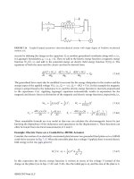
Using Stokes’s theorem, one has
or
The electromagnetic torque T acts on the infinitesimal current loop in a direction to align the magnetic
moment m with the external field B, and if m and B are misaligned by the angle
θ
, we have
The incremental potential energy and work are found as
Using the electromagnetic force, we have
and

Coordinate Systems and Electromagnetic Field
The transformation from the inertial coordinates to the permanent-magnet coordinates is
We use the transformation matrix
If the deflections are small, we have
T i
dA ∇ rB⋅()B ∇ r×()dA⋅
s
∫
°
–×
s
∫
°


idAB×
s
∫
°
==
T iAB× mB×==

TmBqsin=
dW dΠ T dq mB q dq and Wsin Π mB qcos– mB⋅–== = == =
dW dΠ– F dr⋅∇Πdr⋅–== =
F ∇Π– ∇ mB⋅()m ∇⋅()B== =
r T
r
r =
q
y
q
z
coscos q
y
q
z
sincos q
y
sin–
q
x
q
y
q
z
q
x
q
z
sincos–cossinsin q
x

q
y
q
z
q
x
q
z
sincos+sinsinsin q
x
q
y
cossin
q
x
q
y
q
z
q
x
sin q
z
sin+cossincos q
x
q
y
q
z
q

x
q
z
cossin–sinsincos q
x
q
y
coscos
x
y
z
=
r
x
y
z
, r
x
y
z
==
T
r
=
q
y
q
z
coscos q
y

q
z
sincos q
y
sin–
q
x
q
y
q
z
q
x
q
z
sincos–cossinsin q
x
q
y
q
z
q
x
q
z
sincos+sinsinsin q
x
q
y
cossin

q
x
q
y
q
z
q
x
q
z
sinsin+cossincos q
x
q
y
q
z
q
x
q
z
cossin–sinsincos q
x
q
y
coscos
T
rs
1 q
z
−q

y
−q
z
1 q
x
q
y
q–
x
1
=
0066_Frame_C20.fm Page 122 Wednesday, January 9, 2002 1:47 PM
©2002 CRC Press LLC
Using Stokes’s theorem, one has
or
The electromagnetic torque T acts on the infinitesimal current loop in a direction to align the magnetic
moment m with the external field B, and if m and B are misaligned by the angle
θ
, we have
The incremental potential energy and work are found as
Using the electromagnetic force, we have
and

Coordinate Systems and Electromagnetic Field
The transformation from the inertial coordinates to the permanent-magnet coordinates is
We use the transformation matrix
If the deflections are small, we have
T i
dA ∇ rB⋅()B ∇ r×()dA⋅
s

∫
°
–×
s
∫
°


idAB×
s
∫
°
==
T iAB× mB×==
TmBqsin=
dW dΠ T dq mB q dq and Wsin Π mB qcos– mB⋅–== = == =
dW dΠ– F dr⋅∇Πdr⋅–== =
F ∇Π– ∇ mB⋅()m ∇⋅()B== =
r T
r
r =
q
y
q
z
coscos q
y
q
z
sincos q

y
sin–
q
x
q
y
q
z
q
x
q
z
sincos–cossinsin q
x
q
y
q
z
q
x
q
z
sincos+sinsinsin q
x
q
y
cossin
q
x
q

y
q
z
q
x
sin q
z
sin+cossincos q
x
q
y
q
z
q
x
q
z
cossin–sinsincos q
x
q
y
coscos
x
y
z
=
r
x
y
z

, r
x
y
z
==
T
r
=
q
y
q
z
coscos q
y
q
z
sincos q
y
sin–
q
x
q
y
q
z
q
x
q
z
sincos–cossinsin q

x
q
y
q
z
q
x
q
z
sincos+sinsinsin q
x
q
y
cossin
q
x
q
y
q
z
q
x
q
z
sinsin+cossincos q
x
q
y
q
z

q
x
q
z
cossin–sinsincos q
x
q
y
coscos
T
rs
1 q
z
−q
y
−q
z
1 q
x
q
y
q–
x
1
=
0066_Frame_C20.fm Page 122 Wednesday, January 9, 2002 1:47 PM
©2002 CRC Press LLC


IV

Systems and

Controls

21 The Role of Controls in Mechatronics



Job van Amerongen

Introduction • Key Elements of Controlled Mechatronic Systems • Integrated Modeling,
Design and Control Implementation • Modern Examples of Mechatronic Systems in
Action • Special Requirements of Mechatronics that Differentiate from “Classic” Systems
and Control Design

22 The Role of Modeling in Mechatronics Design



Jeffrey A. Jalkio

Modeling as Part of the Design Process • The Goals of Modeling • Modeling of Systems
and Signals

23 Signals and Systems



Momoh-Jimoh Eyiomika Salami, Rolf Johansson,

Kam Leang, Qingze Zou, Santosh Devasia, and C. Nelson Dorny

Continuous and Discrete-Time Signals •

z

Transform and Digital Systems • Continuous-
and Discrete-Time State-Space Models • Transfer Functions and Laplace Transforms

24 State Space Analysis and System Properties



Mario E. Salgado and Juan I. Yuz

Models: Fundamental Concepts • State Variables: Basic Concepts • State Space Description
for Continuous-Time Systems • State Space Description for Discrete-Time and Sampled
Data Systems • State Space Models for Interconnected Systems • System Properties • State
Observers • State Feedback • Observed State Feedback

25 Response of Dynamic Systems



Raymond de Callafon

System and Signal Analysis • Dynamic Response • Performance Indicators for
Dynamic Systems

26 The Root Locus Method

Hitay Özbay

Introduction • Desired Pole Locations • Root Locus Construction • Complementary Root
Locus • Root Locus for Systems with Time Delays • Notes and References

27 Frequency Response Methods



Jyh-Jong Sheen

Introduction • Bode Plots • Polar Plots • Log-Magnitude Versus Phase
plots • Experimental Determination of Transfer Functions • The Nyquist Stability
Criterion • Relative Stability

28 Kalman Filters as Dynamic System State Observers



Timothy P. Crain II

The Discrete-Time Linear Kalman Filter • Other Kalman Filter Formulations •
Formulation Summary and Review • Implementation Considerations
©2002 CRC Press LLC


In the initial conceptual design phase it has to be decided which problems should be solved mechan-

ically and which problems electronically. In this stage decisions about the dominant mechanical properties
have to be made, yielding a simple model that can be used for controller design. Also a rough idea about
the necessary sensors, actuators, and interfaces has to be available in this stage. When the different partial
designs are worked out in some detail, information about these designs can be used for evaluation of
the complete system and be exchanged for a more realistic and detailed design of the different parts.
Although the word mechatronics is new, mechatronic products have been available for some time. In
fact, all electronically controlled mechanical systems are based on the idea of improving the product by
adding features realized in another domain. Good mechatronic designs are based on a

real systems
approach

. But mostly, control engineers are confronted with a design in which major parameters are
already fixed, often based on static or economic considerations. This prohibits optimization of the system
as a whole, even when optimal control is applied.
In the last days of gramophones, the more sophisticated designs used tacho feedback in combination
with a light turntable to achieve a constant number of revolutions. But a really new design was the
compact disc player. Instead of keeping the number of revolutions of the disc constant, it aims for a
constant speed of the head along the tracks of the disc. This means that the disc rotates slower when
tracks with a greater diameter are read. The bits read from the CD are buffered electronically in a buffer
that sends its information to the DA converter, controlled by a quartz crystal. This enables the realization
of a very constant bit rate and eliminates all audible speed fluctuations. Such a performance could never
be obtained from a pure mechanical device only, even if it were equipped with a good speed control
system. In fact, the control loop for the disc speed does not need to have very strict specifications. It
should only prevent overflow or underflow of the buffer. The high accuracy is obtained in an open loop
mode, steered by a quartz crystal (Fig. 21.3).
The flexibility introduced by the combination of precision mechanics and electronic control has
allowed the development of CD-ROM players, running at speeds more than 50 times faster than the
original audio CDs. A new way of thinking was necessary to come to such a new solution. On the other
hand, the CD player is still a sophisticated piece of precision mechanics. No solid-state electronic memory

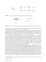
FIGURE 21.1

Optimization of the controller.

FIGURE 21.2

Optimization of the all system components simultaneously.
©2002 CRC Press LLC